
TD - Multiple regressions
Aurélien Ginolhac, Eric Koncina
2019-11-21
Interaction between predictors
In the lecture12, we used the advertising dataset and retained the following linear model:
\[\widehat{Sales} = \hat{\beta_0} + \hat{\beta_1} TV + \hat{\beta_2} Radio + \hat{\beta_3} (TV:Radio)\]
Load the data and perform the linear regression
Load the data set again (you can download it from here)
advert <- read_csv("https://biostat2.uni.lu/practicals/data/advertising.csv",
                   col_types = cols(
                     .default = col_double(),
                     obs = col_integer()))
Perform the multiple linear regression with 3 predictors and interaction and store it in an object called adv_lm.
adv_lm <- lm(Sales ~ TV * Radio, data = advert)Writing the equation associated to the linear regression
Now, using formula in the red box above, we would like to explicitely formulate this linear model using the estimated coefficients. For example, let’s consider the following hypothetical linear model \(y = a \times x + b\) with the estimates \(a = 2\) and \(b = 1\). We would write it as \(y = 2 \times x + 1\).
Extract the coefficients and round the values to 3 digits after the decimal point.
# Use coef() to extract the coefficients as a named vector:
coef(adv_lm)
## (Intercept) TV Radio TV:Radio
## 6.750220203 0.019101074 0.028860340 0.001086495# Use round() to ajust the digit number:
(adv_coef <- round(coef(adv_lm), 3))## (Intercept) TV Radio TV:Radio
## 6.750 0.019 0.029 0.001Write down the equation associated to the linear model using the estimated coefficients.
Tip
glue::glue() to generate the equation in R
# Lets create some example objects
a <- 2
b <- 1

# The following line will not modify our character sequence:
glue::glue("y = a * x + b")
## y = a * x + b# character sequences surrounded by curly braces are detected
# as R objects and replaced by their values
glue::glue("y = {a} * x + {b}")## y = 2 * x + 1glue::glue("sales = {adv_coef['(Intercept)']} + TV * {adv_coef['TV']} + Radio * { adv_coef['Radio']} + (TV:Radio) * {adv_coef['TV:Radio']}")## sales = 6.75 + TV * 0.019 + Radio * 0.029 + (TV:Radio) * 0.001Can you reject the null hypothesis for each coefficient?
tidy(adv_lm). Thus, the null hypothesis can be rejected and we conclude that all coefficients are significantly different from zero.
Rewrite the equation (by hand) and factorise \(TV\), i. e such as \(TV\times(\hat{\beta_1} + x \times Radio)\)
sales = 6.75 + TV * 0.019 + Radio * 0.029 + (TV * Radio) * 0.001
sales = 6.75 + TV * (0.019 + 0.001 * Radio) + Radio * 0.029
We would like to invest 2 units (2000$) in advertisings.
Using the factorised equation quickly determine whether it is better:
- to invest all the money in TV
- to invest all the money in Radio
- invest in both media
sales = 6.75 + TV * (0.019 + 0.001 * Radio) + Radio * 0.029
- radio only: \(sales \approx 1000 \times 0.029 \ll 1000\) (6.75 + 0 * (0.019 + 0.001 * 2000) + 2000 * 0.029 = 64.75)
- TV only: \(sales \approx 1000 \times 0.019 \ll 1000\) (6.75 + 2000 * (0.019 + 0.001 * 0) + 0 * 0.029 = 44.75)
- both: \(sales \approx 1000 \times 1\) (6.75 + 1000 * (0.019 + 0.001 * 1000) + 1000 * 0.029 = 1054.75)
Using R and the fitted model, predict the increase in sales for an investment of 1000$ in TV and 1000$ in Radio.
predict(adv_lm, tibble(TV = 1000, Radio = 1000))## 1
## 1141.206# different value from yours because of rounding issues.Similarly, predict the increase in sales for an investment of 2000$ in TV without any investment in Radio.
Calculate the ratio of the sales when investing in both media to TV alone.
Tip
predict(). And supply as argument a data.frame/tibble where colnames are predictor names and values the desired investment to test
predict(adv_lm, tibble(TV = 2000, Radio = 0))## 1
## 44.95237# Ratio (splitting investment) / (TV only):
predict(adv_lm, data_frame(TV = 1000, Radio = 1000)) / predict(adv_lm, data_frame(TV = 2000, Radio = 0))## Warning: `data_frame()` is deprecated, use `tibble()`.
## This warning is displayed once per session.## 1
## 25.38701Fitting the model without interaction
Create a new model in R explaining the \(sales\) by the investment in \(TV\) and \(Radio\) but without an interaction.
adv_lm2 <- lm(Sales ~ TV + Radio, data = advert)Extract the coefficients
adv_coef2 <- coef(adv_lm2)

(adv_coef2 <- round(adv_coef2, 3))
## (Intercept) TV Radio
## 2.921 0.046 0.188Write the equation associated to the model using the predicted coefficients
glue::glue("sales = {adv_coef2['(Intercept)']} + TV * {adv_coef2['TV']} + Radio * { adv_coef2['Radio']}")## sales = 2.921 + TV * 0.046 + Radio * 0.188Quickly compare this equation to the factorised one in the previous question.
Do you think that the efficiency of investing 2000$ will be similar in both models?
sales = 2.921 + TV * 0.046 + Radio * 0.188
When investing (2000 $) the sales won’t be as high as in the model with interaction.
Using the model without interaction and R, predict the increase in sales for an investment of 1000$ in TV and 1000$ in Radio.
predict(adv_lm2, tibble(TV = 1000, Radio = 1000))## 1
## 236.6701Similarly (using the model without interaction), predict the increase in sales for an investment of 2000 $ in TV only.
Calculate the ratio of the sales when investing in both media to TV alone.
predict(adv_lm2, tibble(TV = 2000, Radio = 0))## 1
## 94.43073# Ratio (splitting investment) / (TV only):
predict(adv_lm2, tibble(TV = 1000, Radio = 1000)) / predict(adv_lm2, tibble(TV = 2000, Radio = 0))## 1
## 2.506283Conclude
Simulated data
We are going to manipulate data where the relationship between the variables is simulated. This example comes from Gareth et al. 2013.
Generate the data
Use the following code to generate the data:
set.seed(1)
simul1 <- tibble(x1 = runif(100),
                     x2 = 0.5 * x1 + rnorm(100) / 10,
                     y  = 2 + 2 * x1 + 0.3 * x2 + (rnorm(100)))
variable y is using a linear model
+ write the equation (as text in your markdown document)
+ write the regression coefficients (as text in your markdown document)\(y = \beta_0 + \beta_1 x1 + \beta_2 x2\)
where:
- \(\beta_0 = 2\)
- \(\beta_1 = 2\)
- \(\beta_2 = 0.3\)
Plot the relationship between x1 and x2. You might want to display all relationships using ggpairs
Tip
ggpairs comes from the package GGally
GGally::ggpairs(simul1)## Registered S3 method overwritten by 'GGally':
## method from
## +.gg ggplot2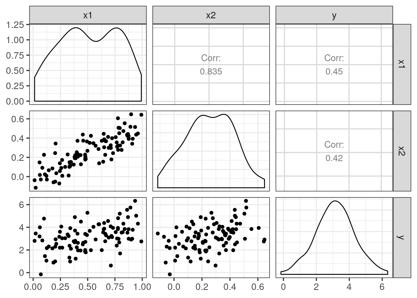
What is the Pearson’s correlation coefficient between x1 and x2?
# we saw it on ggpairs 0.835
cor(simul1$x1, simul1$x2)
## [1] 0.8351212Will the correlation between predictors be a problem for the linear regression you just wrote down?
Name this effect.
Fit a linear model explaining y by x1 + x2 and describe the summary results.
Do you accept \(H_0: \hat{\beta_1} = 0\) and \(H_0: \hat{\beta_2} = 0\)?
lm(y ~ x1 + x2, data = simul1) %>% summary()##
## Call:
## lm(formula = y ~ x1 + x2, data = simul1)
##
## Residuals:
## Min 1Q Median 3Q Max
## -2.8311 -0.7273 -0.0537 0.6338 2.3359
##
## Coefficients:
## Estimate Std. Error t value Pr(>|t|)
## (Intercept) 2.1305 0.2319 9.188 7.61e-15 ***
## x1 1.4396 0.7212 1.996 0.0487 *
## x2 1.0097 1.1337 0.891 0.3754
## ---
## Signif. codes: 0 '***' 0.001 '**' 0.01 '*' 0.05 '.' 0.1 ' ' 1
##
## Residual standard error: 1.056 on 97 degrees of freedom
## Multiple R-squared: 0.2088, Adjusted R-squared: 0.1925
## F-statistic: 12.8 on 2 and 97 DF, p-value: 1.164e-05# both predictors are not significant exhibiting a very high standard error
# due to collinearity. We have to accept the null hypothesis for both x1 and x2
# while we know the true relationship.Fit a linear model explaining y by x1 alone.
Do you accept \(H_0: \hat{\beta_1} = 0\)?
What happened?
lm(y ~ x1 , data = simul1) %>% summary()##
## Call:
## lm(formula = y ~ x1, data = simul1)
##
## Residuals:
## Min 1Q Median 3Q Max
## -2.89495 -0.66874 -0.07785 0.59221 2.45560
##
## Coefficients:
## Estimate Std. Error t value Pr(>|t|)
## (Intercept) 2.1124 0.2307 9.155 8.27e-15 ***
## x1 1.9759 0.3963 4.986 2.66e-06 ***
## ---
## Signif. codes: 0 '***' 0.001 '**' 0.01 '*' 0.05 '.' 0.1 ' ' 1
##
## Residual standard error: 1.055 on 98 degrees of freedom
## Multiple R-squared: 0.2024, Adjusted R-squared: 0.1942
## F-statistic: 24.86 on 1 and 98 DF, p-value: 2.661e-06# now that collinearity is removed, x1 is found with ~ the right coefficient 2
# and std.error was divided by > 2
# we don't find the right coefficient because all variance are spread into one (x1)Fit a linear model explaining y by x2 alone.
Do you accept \(H_0: \hat{\beta_1} = 0\)?
What happened?
lm(y ~ x2 , data = simul1) %>% summary()##
## Call:
## lm(formula = y ~ x2, data = simul1)
##
## Residuals:
## Min 1Q Median 3Q Max
## -2.62687 -0.75156 -0.03598 0.72383 2.44890
##
## Coefficients:
## Estimate Std. Error t value Pr(>|t|)
## (Intercept) 2.3899 0.1949 12.26 < 2e-16 ***
## x2 2.8996 0.6330 4.58 1.37e-05 ***
## ---
## Signif. codes: 0 '***' 0.001 '**' 0.01 '*' 0.05 '.' 0.1 ' ' 1
##
## Residual standard error: 1.072 on 98 degrees of freedom
## Multiple R-squared: 0.1763, Adjusted R-squared: 0.1679
## F-statistic: 20.98 on 1 and 98 DF, p-value: 1.366e-05# now that collineary is removed, x2 is found with ~ the right coefficient 2
# and std.error was divided by > 2One observation was unfortunately forgotten and is: x1 = 0.1, x2 = 0.8, y = 6.
Add it to the existing simul1 and store the result as simul2.
Tip
add_row() defined in the package tibble
simul2 <- add_row(simul1, x1 = 0.1, x2 = 0.8, y = 6)Plot the relationship between x1 and x2 again using the updated dataset simul2.
GGally::ggpairs(simul2)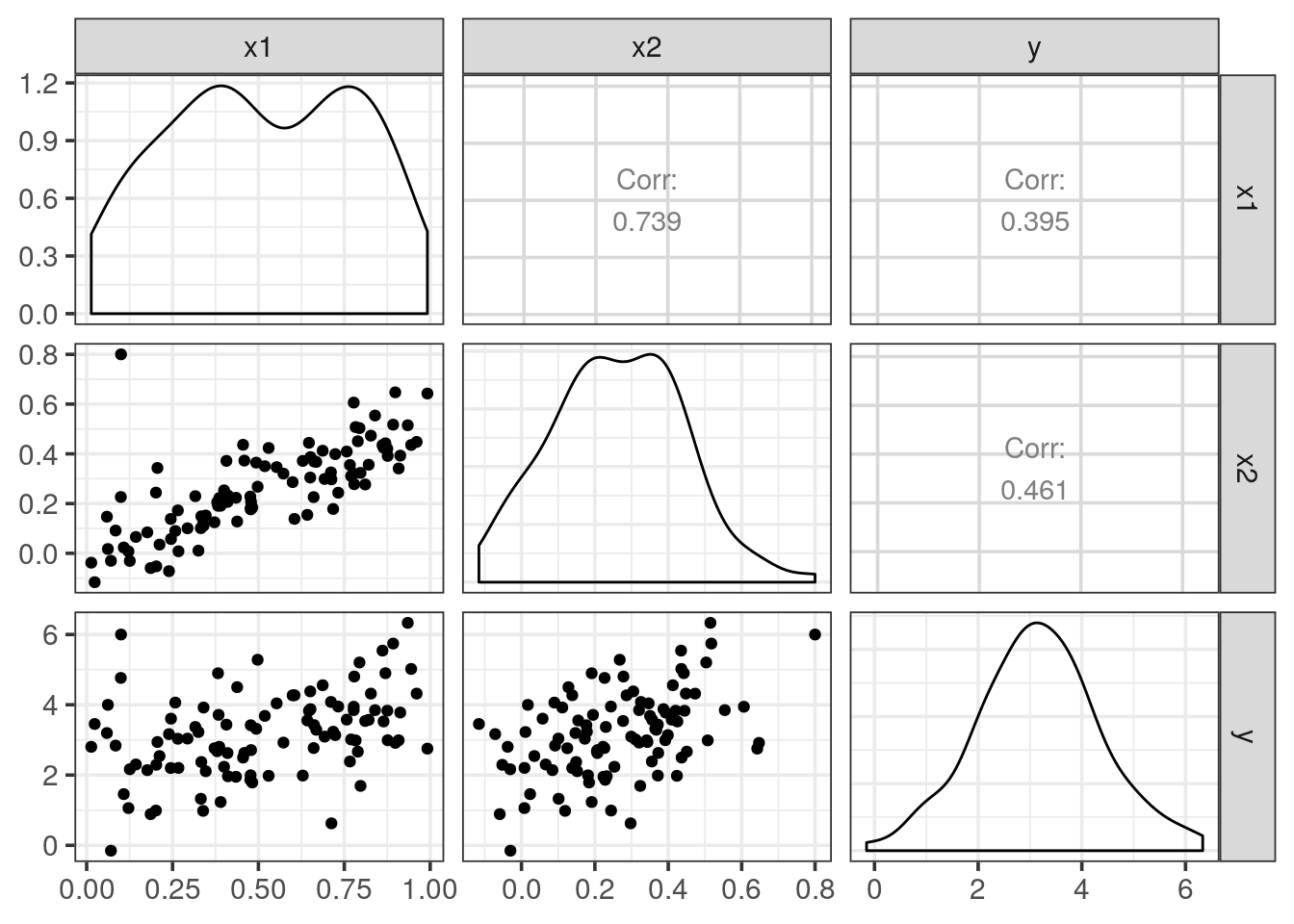
Fit the previous linear model again using simul2
lm(y ~ x1 + x2, data = simul2) %>% summary()##
## Call:
## lm(formula = y ~ x1 + x2, data = simul2)
##
## Residuals:
## Min 1Q Median 3Q Max
## -2.73348 -0.69318 -0.05263 0.66385 2.30619
##
## Coefficients:
## Estimate Std. Error t value Pr(>|t|)
## (Intercept) 2.2267 0.2314 9.624 7.91e-16 ***
## x1 0.5394 0.5922 0.911 0.36458
## x2 2.5146 0.8977 2.801 0.00614 **
## ---
## Signif. codes: 0 '***' 0.001 '**' 0.01 '*' 0.05 '.' 0.1 ' ' 1
##
## Residual standard error: 1.075 on 98 degrees of freedom
## Multiple R-squared: 0.2188, Adjusted R-squared: 0.2029
## F-statistic: 13.72 on 2 and 98 DF, p-value: 5.564e-06