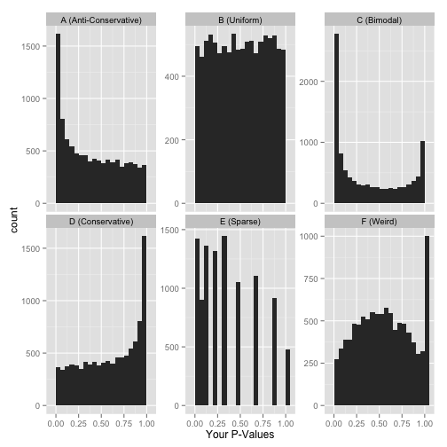
Multiple testing / multiple regressions

November 2019

Learning objectives

You will learn to:

on p-values
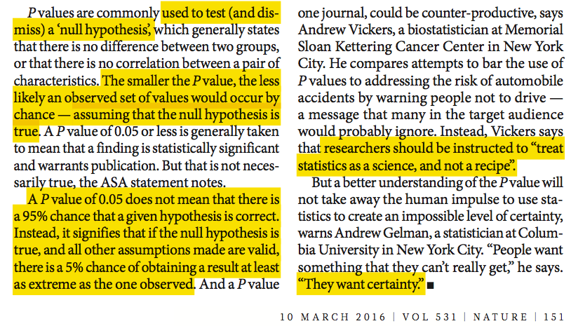
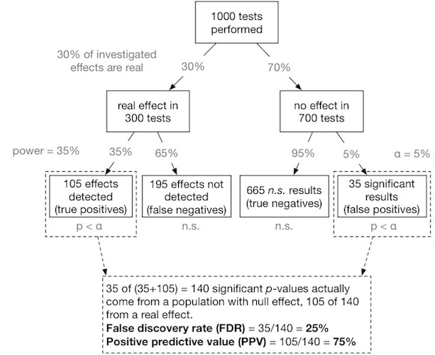
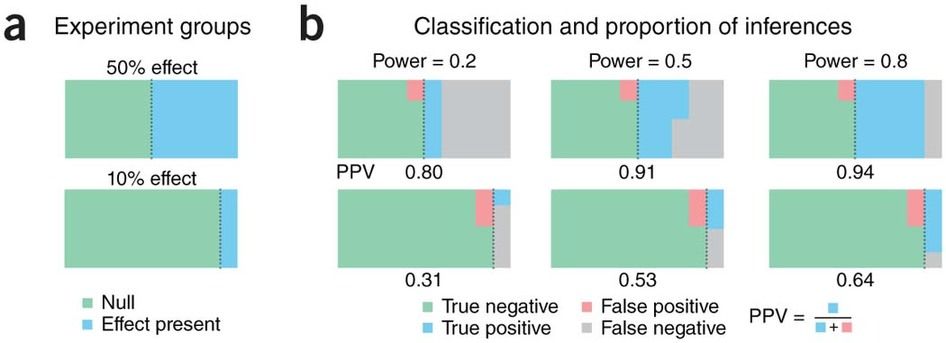
- know what a p-value actually is
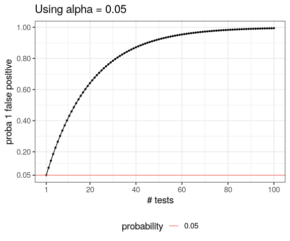
- understand necessity to correct for multiple testing
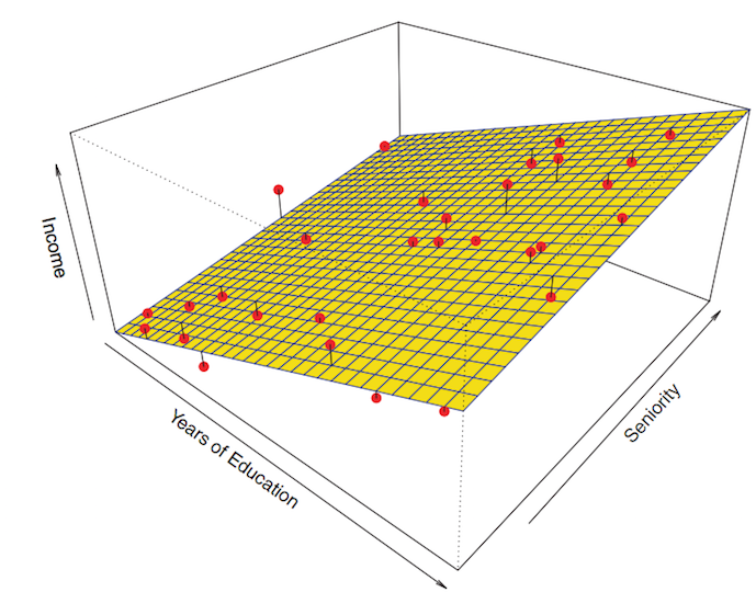
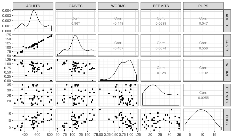
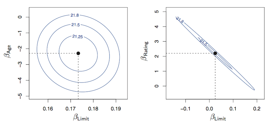
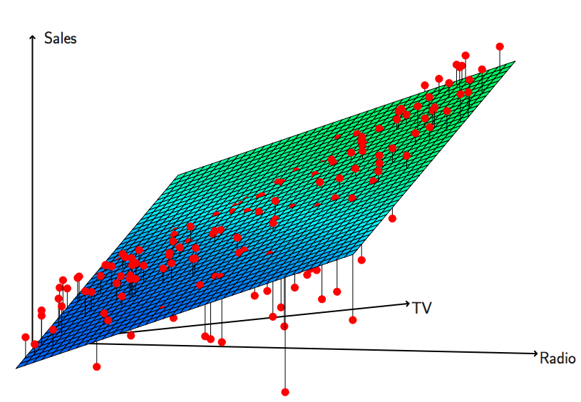
on multiple regression
- how different from simple regression
- model simplification
- testing for predictor interaction
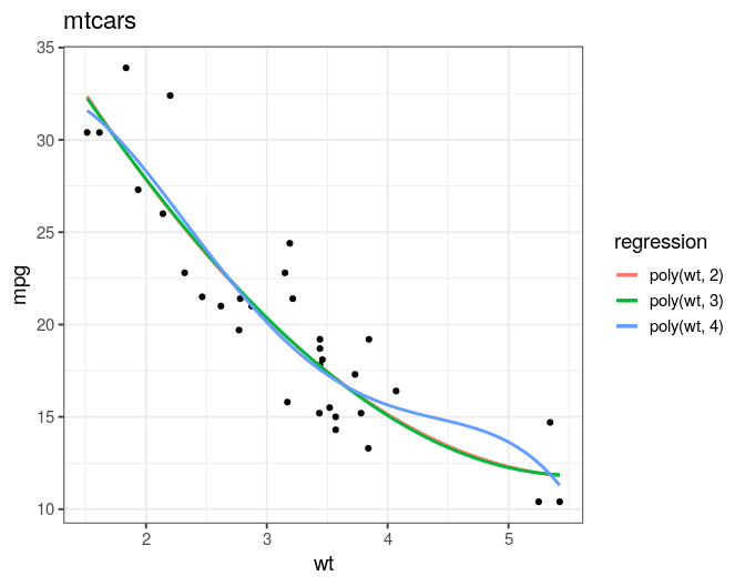
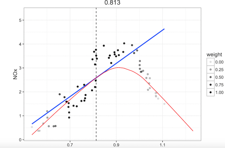
transforming predictor to seek linearity
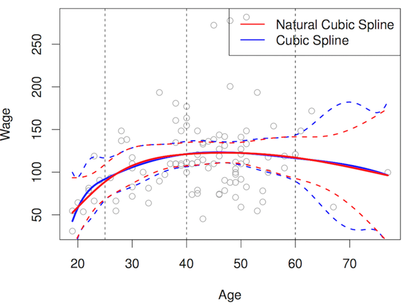
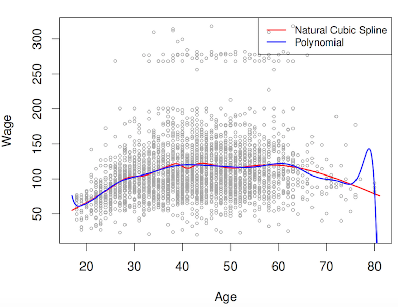
smoothing predictors

Reading

An Introduction to Statistical Learning by James, Witten, Hastie & Tibshirani

Multiple testing

The problem

\[P(Making\ an\ error) = \alpha\] \[P(Not\ making\ an\ error) = 1 - \alpha\] \[P(Not\ making\ an\ error\ in\ m\ tests) = (1 - \alpha)^m\] \[P(Making\ at\ least\ 1\ error\ in\ m\ tests) = 1 - (1 - \alpha)^m\]

Multiple testing

Visualising the problem

# Using alpha = 0.05
tibble(x = 1:100,
       y = map_dbl(x, ~ 1 - (1 - 0.05)^.x)) %>% 
  ggplot(aes(x, y)) +
  geom_point(size = 0.8) +
  geom_line() +
  geom_hline(aes(colour = "0.05",
                 yintercept = 0.05)) +
  labs(x = "# tests",
       y = "proba 1 false positive",
       colour = "probability",
       title = "Using alpha = 0.05") +
  theme(legend.position = "bottom") +
  scale_x_continuous(breaks = c(1, seq(20, 100, 20))) +
  scale_y_continuous(breaks = c(0.05, seq(0.2, 1, 0.2)))

reference: Joshua Akey, University of Washington

what is a p value?

Do you agree with the following?

A p-value is the probability that the null hypothesis is true.

Wrong!

If something is unlikely under the null distribution, it might be less unlikely under the alternative distribution. That is why we are interested in small p-values.[…]
Under the null hypothesis, it is exactly as likely to observe a p-value of 0.99 as a p-value of \(10^{-99}\). Thomas Mailund

under the null hypothesis, p-values are uniformally distributed

sample 100,000 random number from the normal distribution
compute their corresponding p-values
draw the histogram of those p-values

tibble(p = pnorm(rnorm(100000))) %>%
  ggplot(aes(x = p)) +
  geom_histogram(boundary = 0, bins = 40,
                 fill = "goldenrod2",
                 color = "black")

Another question / answer from Thomas Mailund

if the p-value is really the probability that the null hypothesis is true then why do we typically only reject the null hypothesis if the p-value is below 5%?

If the p-value was really that, wouldn’t we go for all p-values below 50%? […] The reason we are interested in low p-values is because if we sample from a mixture of the null distribution and the alternative distribution, then we expect more of the alternatives in the low end of p-values than we expect from the null.

Definition

A p value is the proportion of times that you would see evidence stronger than what was observed, against the null hypothesis, if the null hypothesis were true and you hypothetically repeated the experiment (sampling of individuals from a population) a large number of times. Matthew Stephens

Warning from the American Statistical Association

Statisticians issue warning on P values

Monya Baker 2016

In the real world

Positive Predictive Value

We deal with a mixture of null and alternative hypotheses.

source: Felix Schönbrodt’s blog

Mixture of hypotheses and power of tests

PPV

When unlikely hypotheses are tested, most positive results of underpowered studies can be wrong.source: Krzywinski & Altman 2013

source: Krzywinski & Altman 2013

p-values histogram

David Robinson

First thing to do, before correcting for multiple testing

Great post by David Robinson, broom’s author

Mixture of hypotheses comes in different proportions

David Robinson

blog’s post by David Robinson

p-hacking

What does this function do?

p_hacking <- function(n = 100,
                      pvalue = 1,
                      hack = 0.05) {
  data <- rnorm(n)
  attempts <- 0
  while (pvalue > hack) {
    attempts <- attempts + 1
    cases <- sample(data, n / 2)
    controls <- data[!data %in% cases]
    pvalue <- t.test(cases, controls)$p.value
  }
  return(list(pvalue   = pvalue,
              attempts = attempts))
}

RT @jessenleon #howToAchieveScientificSuccess in 10 lines of #R code!
Tags: #bioinformatics #Rstats #programming pic.twitter.com/dmtlvzZRBO
— Lucasoft co.uk (@lucasoft_co_uk) 24 octobre 2016

modified from lucasoft_co_uk’s tweet

p-hacking

plot

set.seed(123)
tibble(x = 1:100,
           y = map(x, p_hacking, n = 100),
           pvalue = map_dbl(y, "pvalue"),
           attempts = map_dbl(y, "attempts")) %>%
  ggplot(aes(x = attempts)) +
  geom_histogram(bins = 40, fill = "goldenrod2") +
  geom_vline(aes(xintercept = median(attempts)),
             linetype = "dashed") +
  # x labels every 10
  scale_x_continuous(breaks = seq(0, 100, 10)) +
  # no space between x-axis and bars
  scale_y_continuous(expand = c(0, 0))

p-hacking

shiny app by Felix Schönbrodt

Run the shiny app locally

# install.packages(c("shiny", "shinythemes", "shinyBS", "mvtnorm"))
shiny::runGitHub("p-hacker", "nicebread", subdir = "p-hacker")

p-hacker: Train your p-hacking skills!
- app
- code

source: Schönbrodt, F. D. (2016). p-hacker: Train your p-hacking skills! Retrieved from http://shinyapps.org/apps/p-hacker/.

Bonferroni

Crude correction, divide all p values by the number of tests. Very conservative.

\[P(one\; false\; positive) = 1 - (1 - \frac{0.05}{20})^{20}\]

which gives for 20 tests: 0.0488301

For high number of tests (like 20 k), gives inacceptable number of false negatives

\[p\; corrected = \frac{0.05}{20000} = 2.5\times 10^{-6}\]

Controling Type I error leads to a huge type II error

False Discovery Rate

\(m_0\) number of true null hypothesis, unknown
\(m - m_0\) number of true alternative hypotheses
R number of rejected null hypotheses

Sign.	\(H_0\) True	\(H_0\) False	Total
Not significant	Correct	Type II	m - R
Significant	Type I	Correct	R
\(m_0\)	\(m - m_0\)	\(m\)

\[FDR = \frac{Type\; I}{R}\]

controlling false positive among significant results

Example

Fake data with 10% from the alternative hypothesis

set.seed(341)
my_p <- tibble(x = c(rnorm(900),
                     rnorm(100, mean = 3)), 
               p = 1 - pnorm(x),
               real_effect = c(rep(FALSE, 900),
                               rep(TRUE, 100)))
# could pnorm(x, lower.tail = FALSE)

pivot_longer(my_p, names_to = "key",
       values_to = "value", cols = -real_effect) %>%
  ggplot(aes(x = value, y = stat(density))) +
  geom_histogram(bins = 40,
                 boundary = 0,
                 fill = "goldenrod2",
                 colour = "goldenrod2") +
  geom_density() +
  facet_wrap(~ key, scales = "free", ncol = 1)

No correction for multiple testing

count significant

my_p %>% 
  mutate(significant = p < 0.05) %>%
  count(real_effect, significant)

# A tibble: 4 x 3
  real_effect significant     n
  <lgl>       <lgl>       <int>
1 FALSE       FALSE         852
2 FALSE       TRUE           48
3 TRUE        FALSE           6
4 TRUE        TRUE           94

which gives

type I error: \(\alpha = \frac{48}{852 + 48} = 0.053\)
type II error: \(\beta = \frac{6}{6 + 94} = 0.06\)
\(power = (1 - \beta) = 0.94\)
\(FDR = \frac{48}{48 + 94} = 0.34\)
\(PPV = 1 - FDR = 0.66\)

should we accept such values?

With Bonferroni correction

Count significant p-values

my_p %>% 
  mutate(significant = p < 0.05 / 1000) %>%
  count(real_effect, significant) %>%
  complete(real_effect, significant, fill = list(n = 0))

# A tibble: 4 x 3
  real_effect significant     n
  <lgl>       <lgl>       <dbl>
1 FALSE       FALSE         900
2 FALSE       TRUE            0
3 TRUE        FALSE          76
4 TRUE        TRUE           24

Using R and `p.adjust()`

my_p %>% 
  mutate(
    p_adj = p.adjust(p, method = "bonferroni"),
    significant = p_adj < 0.05
    ) %>%
  count(real_effect, significant)

which gives

type I error: \(\alpha = \frac{0}{900 + 0} = 0\)
type II error: \(\beta = \frac{76}{76 + 24} = 0.76\)
\(power = (1 - \beta) = 0.24\)
\(FDR = \frac{0}{0 + 24} = 0\)
\(PPV = 1 - FDR = 1\)

should we accept such values?

With Benjamini & Hochberg correction

False Discovery Rate

Count significant p-values

my_p %>% 
  mutate(
    significant = map_lgl(
      p, ~ .x < match(.x, sort(p)) * 0.05 / 1000
      )
    ) %>%
  count(real_effect, significant)

# A tibble: 4 x 3
  real_effect significant     n
  <lgl>       <lgl>       <int>
1 FALSE       FALSE         897
2 FALSE       TRUE            3
3 TRUE        FALSE          43
4 TRUE        TRUE           57

Using R and `p.adjust()`

my_p %>% 
  mutate(p_adj = p.adjust(p, method = "BH"),
         # same as method = "fdr"
         significant = p_adj < 0.05) %>%
  count(real_effect, significant)

which gives

type I error: \(\alpha = \frac{3}{897 + 3} = 0.003\)
type II error: \(\beta = \frac{43}{43 + 57} = 0.43\)
\(power = (1 - \beta) = 0.57\)
\(FDR = \frac{3}{3 + 57} = 0.05\)
\(PPV = 1 - FDR = 0.95\)

q values

John Storey & Robert Tibshirani

Using the `qvalue` library

The goal is to estimate the proportion of \(\pi_0\) of null (BH uses \(\pi_0 = 1\))
See package info at github and shiny app

#source("http://bioconductor.org/biocLite.R")
#biocLite("qvalue")
library(qvalue)
my_p %>% 
  mutate(q_val = qvalue(p)$qvalues,
         significant = q_val < 0.05) %>%
  count(real_effect, significant)

# A tibble: 4 x 3
  real_effect significant     n
  <lgl>       <lgl>       <int>
1 FALSE       FALSE         897
2 FALSE       TRUE            3
3 TRUE        FALSE          43
4 TRUE        TRUE           57

which gives

type I error: \(\alpha = \frac{3}{897 + 3} = 0.003\)
type II error: \(\beta = \frac{43}{43 + 57} = 0.43\)
\(power = (1 - \beta) = 0.57\)
\(FDR = \frac{3}{3 + 57} = 0.05\)
\(PPV = 1 - FDR = 0.95\)

q values

true example

False Positive Rate and False Discovery Rate

the false positive rate is the rate that truly null features are called significant. The FDR is the rate that significant features are truly null. For example, a false positive rate of 5% means that on average 5% of the truly null features in the study will be called significant. A FDR of 5% means that among all features called significant, 5% of these are truly null on average.Storey and Tibshirani 2003

multiple linear regression

Extend the simple linear regression

Gives each p predictor a separate slope coefficients and \(\beta_0\) is the intercept

\[Y = \beta_0 + \beta_1 \times X_1 + \beta_2 \times X_2 + \ldots + \beta_p \times X_p + \epsilon\]

separate simple versus multiple regressions

Advertising example

separate linear

media	term	estimate	p.value
Newspaper	(Intercept)	12.351	4.71e-49
Newspaper	slope	0.055	1.15e-03
Radio	(Intercept)	9.312	3.56e-39
Radio	slope	0.202	4.35e-19
TV	(Intercept)	7.033	1.41e-35
TV	slope	0.048	1.47e-42

multiple linear

term	estimate	p.value
(Intercept)	2.939	1.27e-17
TV	0.046	1.51e-81
Radio	0.189	1.51e-54
Newspaper	-0.001	8.60e-01

Newspaper is not longer significant

Fake effect due to a masked variable

correlation matrix

GGally::ggpairs(select(advert, -obs))

Newspaper gets hooked by Radio, R = 0.35 is enough

Collinearity

Variance Inflation Factor

variance when removed

\(VIF = \frac{1}{1 - R^2_{X_j|X_{-j}}}\)

smallest possible value is 1

the library `car` provides such estimate

rule of a thumb:

> 5 means troubles
> 10 means BIG troubles

adverstising

car::vif(lm(Sales ~ TV + Radio + Newspaper, data = advert))

       TV     Radio Newspaper 
 1.004611  1.144952  1.145187

another example

read_csv("data/WOLFPUPS.csv") %>%
  lm(PUPS ~ ADULTS + CALVES + WORMS + PERMITS, data = .) %>% car::vif()

   ADULTS    CALVES     WORMS   PERMITS 
15.592589 15.387900  1.266965  1.016862

when multicollinearity occurs, watching pairs is not enough, use VIF

Collinearity, when strong

correlation matrix

Collinearity

effect on coefficient

From ISLR, James, Witten, Hastie & Tibshirani

The F statistic

Is any of the predictors having an effect on the response?

Call:
lm(formula = Sales ~ TV + Radio + Newspaper, data = .)

Residuals:
    Min      1Q  Median      3Q     Max 
-8.8277 -0.8908  0.2418  1.1893  2.8292 

Coefficients:
             Estimate Std. Error t value Pr(>|t|)    
(Intercept)  2.938889   0.311908   9.422   <2e-16 ***
TV           0.045765   0.001395  32.809   <2e-16 ***
Radio        0.188530   0.008611  21.893   <2e-16 ***
Newspaper   -0.001037   0.005871  -0.177     0.86    
---
Signif. codes:  0 '***' 0.001 '**' 0.01 '*' 0.05 '.' 0.1 ' ' 1

Residual standard error: 1.686 on 196 degrees of freedom
Multiple R-squared:  0.8972,    Adjusted R-squared:  0.8956 
F-statistic: 570.3 on 3 and 196 DF,  p-value: < 2.2e-16

\[F = \frac{(TSS - RSS) / p}{RSS / (n - p -1)}\]

F takes the number of predictors p into account

Otherwise, for 100 p and \(\alpha=0.05\), we expect 5 individuals slopes to be significant by chance!

Model simplification

backward or forward

backward

re(lm(Sales ~ TV + Radio + Newspaper,
      data = advert))

# A tibble: 1 x 4
  r.squared adj.r.squared df.residual    df
      <dbl>         <dbl>       <int> <int>
1     0.897         0.896         196     4

re(lm(Sales ~ TV + Radio, data = advert))

# A tibble: 1 x 4
  r.squared adj.r.squared df.residual    df
      <dbl>         <dbl>       <int> <int>
1     0.897         0.896         197     3

re(lm(Sales ~ TV, data = advert))

# A tibble: 1 x 4
  r.squared adj.r.squared df.residual    df
      <dbl>         <dbl>       <int> <int>
1     0.612         0.610         198     2

test if removing Newspaper is significant

anova(lm(Sales ~ TV + Radio + Newspaper, data = advert), lm(Sales ~ TV + Radio, data = advert))

Analysis of Variance Table

Model 1: Sales ~ TV + Radio + Newspaper
Model 2: Sales ~ TV + Radio
  Res.Df    RSS Df Sum of Sq      F Pr(>F)
1    196 556.83                           
2    197 556.91 -1 -0.088717 0.0312 0.8599

forward is mandatory, if p predictors is > n

3D plot of 2 predictors

without interaction

Interaction between predictors

additional coefficient

\[Y = \beta_0 + \beta_1 \times X_1 + \beta_2 \times X_2 + \beta_3 \times X_1X_2 + \epsilon\]

re(lm(Sales ~ TV + Radio, data = advert))

# A tibble: 1 x 4
  r.squared adj.r.squared df.residual    df
      <dbl>         <dbl>       <int> <int>
1     0.897         0.896         197     3

re(lm(Sales ~ TV * Radio, data = advert))

# A tibble: 1 x 4
  r.squared adj.r.squared df.residual    df
      <dbl>         <dbl>       <int> <int>
1     0.968         0.967         196     4

detailed output

tidy(lm(Sales ~ TV * Radio, data = advert))

# A tibble: 4 x 5
  term        estimate std.error statistic  p.value
  <chr>          <dbl>     <dbl>     <dbl>    <dbl>
1 (Intercept)  6.75    0.248         27.2  1.54e-68
2 TV           0.0191  0.00150       12.7  2.36e-27
3 Radio        0.0289  0.00891        3.24 1.40e- 3
4 TV:Radio     0.00109 0.0000524     20.7  2.76e-51

Hierarchy principle

It could happen that the interaction term is significant but not the main effects

in Adverstising example

TV:Radio had a very small p-value
TV nor Radio

the hierachy principle

if we include an interaction we must include the main effects regardless of their individual p-values

formula in R

Model	Formula	Comments
Null	`y ~ 1`	intercept = 1
Simple regression	`y ~ x`	`x` continuous
Multiple regression	`y ~ x + z`	2 continuous predictors
Multiple regression	`y ~ x * z`	2 continuous predictors and interaction
Multiple regression	`y ~ x : z`	interaction between predictors
Multiple regression	`y ~ x + z + x : z`	2 continuous predictors and interaction
Multiple regression	`y ~ x * z - x : z`	2 continuous predictors
one-way ANOVA	`y ~ gender`	one categorical predictor
two-ways ANOVA	`y ~ gender + geno`	2 categorical predictors

adapted from Michael J. Crawley

Beyond linearity

Non-linear

pattern in residuals

linear model, no transformation

lm(mpg ~ wt, data = mtcars) %>%
  augment() %>%
  ggplot(aes(x = .fitted, y = .resid)) +
  geom_point() +
  geom_smooth(method = "loess")

linear model, quadratic transformation

lm(mpg ~ wt + I(wt^2), data = mtcars) %>%
  augment() %>%
  ggplot(aes(x = .fitted, y = .resid)) +
  geom_point() +
  geom_smooth(method = "loess")

Polynomial regression

predictor transformation

\[mpg = \beta_0 + \beta_1 \times weigth + \beta_2 \times weigth^2\]

Seek for linearity in any space

goal: find linearity after transforming the predictors and / or the response

Like in the the diamond example

pattern in residuals could help
if not, use a more flexible model, such as splines or loess
if you failed to find a decent fit, go for non-linear models

Polynomial regression

Is a multiple linear regression with several degrees of the same predictor.

square

select(tidy(mpg_poly2_wt), 1:2)

# A tibble: 3 x 2
  term         estimate
  <chr>           <dbl>
1 (Intercept)     20.1 
2 poly(wt, 2)1   -29.1 
3 poly(wt, 2)2     8.64

select(glance(mpg_poly2_wt), c(1:3, 5, 6))

# A tibble: 1 x 5
  r.squared adj.r.squared sigma  p.value    df
      <dbl>         <dbl> <dbl>    <dbl> <int>
1     0.819         0.807  2.65 1.71e-11     3

cubic

select(tidy(mpg_poly3_wt), 1:2)

# A tibble: 4 x 2
  term         estimate
  <chr>           <dbl>
1 (Intercept)    20.1  
2 poly(wt, 3)1  -29.1  
3 poly(wt, 3)2    8.64 
4 poly(wt, 3)3    0.275

select(glance(mpg_poly3_wt), c(1:3, 5, 6))

# A tibble: 1 x 5
  r.squared adj.r.squared sigma  p.value    df
      <dbl>         <dbl> <dbl>    <dbl> <int>
1     0.819         0.800  2.70 1.58e-10     4

Polynomial regression

plotting

Other transformations, shape in residuals

Banana shape

\(X^2\)
\(poly(X, a)\) where \(a\) is the polynomial degree. Help creating them all
\(\sqrt{X}\)
\(log(X)\)

Funnel shape

\(\sqrt{Y}\)
\(log(Y)\)

Smoothing

regression splines

combine a polynomial fit for k distinct regions of the continuous variable
constraint: regression join smoothly between 2 regions.

local polynomial regression fitting (loess)

default of geom_smooth()
similar as spline but regions are overlapping
allows more smoothing

Cubic splines

`splines::bs()`

Multiple regression with \(\beta1 X + \beta2 X^2 + \beta3 X^3\). Coefs change for every knots of \(X\)

Natural cubic splines

`splines::ns()`

additional constraint on the boundary: must be a linear fit

Natural cubic splines

advantage over polynomial

for high polynomial order, the linear constraint helps

Local Polynomial Regression Fitting

loess

best is the David Robinson animation

regression and overlapping regions using weights.

Before we stop

Acknowledgments

Some of the figures in this presentation are taken from:

An Introduction to Statistical Learning, with applications in R (Springer, 2013) with permission from the authors: G. James, D. Witten, T. Hastie and R. Tibshirani
Biostatistic Design and Analysis Using R. (Wiley-Blackwell, 2011) Murray Logan

People

Hákon Jónsson
Luc Buissière

Learning objectives

You will learn to:

Reading

Multiple testing

The problem

Multiple testing

Visualising the problem

what is a p value?

Do you agree with the following?

under the null hypothesis, p-values are uniformally distributed

Another question / answer from Thomas Mailund

Definition

Warning from the American Statistical Association

Statisticians issue warning on P values

In the real world

Positive Predictive Value

We deal with a mixture of null and alternative hypotheses.

Mixture of hypotheses and power of tests

PPV

p-values histogram

David Robinson

Mixture of hypotheses comes in different proportions

David Robinson

p-hacking

What does this function do?

p-hacking

plot

p-hacking

shiny app by Felix Schönbrodt

Run the shiny app locally

Bonferroni

False Discovery Rate

Example

Fake data with 10% from the alternative hypothesis

No correction for multiple testing

count significant

which gives

With Bonferroni correction

Count significant p-values

Using R and p.adjust()

which gives

With Benjamini & Hochberg correction

False Discovery Rate

Count significant p-values

Using R and p.adjust()

which gives

q values

John Storey & Robert Tibshirani

Using the qvalue library

which gives

q values

true example

False Positive Rate and False Discovery Rate

multiple linear regression

Extend the simple linear regression

separate simple versus multiple regressions

Advertising example

separate linear

multiple linear

Fake effect due to a masked variable

correlation matrix

Collinearity

Variance Inflation Factor

variance when removed

the library car provides such estimate

adverstising

another example

Collinearity, when strong

correlation matrix

Collinearity

effect on coefficient

The F statistic

Is any of the predictors having an effect on the response?

F takes the number of predictors p into account

Model simplification

backward or forward

backward

test if removing Newspaper is significant

3D plot of 2 predictors

without interaction

Using R and `p.adjust()`

Using R and `p.adjust()`

Using the `qvalue` library

the library `car` provides such estimate

`splines::bs()`

`splines::ns()`