
TD data import
Eric Koncina
2019-09-25
In this practical, you’ll learn how to import flat files using the readr package which is part of the tidyverse.
To perform reproducible research it is a good practice to store the files in a standardised location. For example, you could take advantage of the RStudio projects and store data files in a subfolder called data.
If you did not create an Rstudio project for this tutorial start to do it now and create a project named readr_tutorial.
Tip
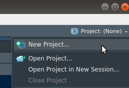
Project icon to create a new one. Once you switched to the project you just created (readr_tutorial) you should see readr_tutorial instead of Project (None).
Before you start
Prepare your project’s folder
Check that the project is active: the name
readr_tutorialshould appear on the top-right corner.Use the
Filespane in the lower right Rstudio panel to create a folder nameddatawithin your project’s folder.Download the files
mtcars.csvandmtcars2.csvand place them in thedatasubfolder you just created. Try to use your operating system’s file browser to place the files at the appropriate location. In that way you’ll get used to the place where your project’s files are located on your computer. If you’re lost try to determine the current working directory which is likely your project’s folder.
Tip
here::here() to determine your project’s root folder.Go to the path showed by one of these commands to find your files.
Load the required library
First load the tidyverse package (which contains readr) or at least load the readr package:
- Add a chunk at the beginning of your document and use
library()to load thetidyverseorreadrpackage. - Don’t forget to run the chunk’s code to load the library during your interactive session (or load the package using the console).
Warning
knit button, the chunks are evaluated in a new environment.
Use readr to load your first file
Now let’s try to load the content of the mtcars.csv file using readr.
- Create a new chunk
- Insert a call to
read_csv()with “data/mtcars.csv” as argument. - Save the result in a new variable called
my_cars.
Tip
?read_csv if you need help.
The tibble
read_csv() loads the data as a tibble. The main advantage to use tibbles over a regular data frame is the printing.
- Go to the console pane and type in
my_cars(followed by Enter). - Tibbles show some useful informations such as the number of rows and columns:
- Look at the top of the tibble and find the information “A tibble rows x cols”
- How many rows are in the tibble?
- The columns of a tibble report their type:
- Look at the tibble header, the type of a columns is reported just below its name.
- What is the type of the
wtcolumn?
However, when unsing RStudio’s inline output, the output is slightly changed: The tibble size is reported at the bottom of the rendered table (which is styled with some navigation options).
- Create a R code chunk in your Rmarkdown document and type in
my_cars. - Execute the chunk to see how Rstudio renders the content of the tibble.
Alternatively you can also click on the object my_cars in the Environment tab of the upper right Rstudio pane where your objects are listed. When you click on the object, RStudio calls View() to open it and view more of the content.
Now you are able to import a simple .csv flat file. csv stands for comma separated values.
Import a “tricky” .csv file
Sometimes importing a file is not as straightforward and needs some adjustments. Download the mtcars2.csv file and try to load it: the file extension is the same, thus we are going to use read_csv() as we did before:
Trying read_csv() again…
- Add a new header in your Rmarkdown and define that you are starting the second part of this tutorial.
- Add a new chunk and read
mtcars2.csvas we did in the previous question:
read_csv(here::here("data", "mtcars2.csv"))Look at the generated tibble: the output is probably not what we would expect…
- It seems that
read_csv()recognized only a single column. - If you look at the column name you’ll see that there is indeed only a single name with all expected names being separated by semicolons instead of the expected commas (remind
csvshould stand for comma separated values).
It turns out that .csv files are not necessary delimited by commas.
Using read_delim()
In fact, read_csv() is a shortcut to a more general readr function which is read_delim().
- Let’s use
read_delim()instead ofread_csv():- Adjust the
delimargument accordingly. - Store the output in an object called
my_cars2
- Adjust the
Tip
?read_delim if you don’t know how to use read_delim
As we assigned the result of the read_delim() function to a new object my_cars, the content (tibble) does not appear on the screen or in the output document. Nevertheless, the message generated by read_delim() is shown (as we didn’t adjust the col_types argument): Now we are able to load mutliple columns again.
Now, let’s look again at the generated output (the tibble):
- Create a chunk below containing only
my_cars2and execute it in order to print the content ofmy_cars2. - You can also type
my_cars2in the console below to get the standardtibbleoutput.
It seems that adjusting the delim argument did it: We get a tibble with the same dimensions as before.
But wait… Something seems different…
Let’s look again at our previous tibble (my_cars). Type again my_cars in the console to print the tibble and compare both outputs.
Look at the mpg colum: the values seem much higher in my_cars2 than in my_cars…
It seems that the decimal separator was not recognized as it should… Maybe it is lacking in the file or something went wrong during the import. As you learned during the lecture, readr guesses the content of each column using some helper functions. To display the content as it is in the file (and avoid any coercion), we can force read_delim to import all the data as text.
- Use the
.defaultargument of thecols()function to apply the setting to all columns.
Tip
read_* functions without adjusting the col_types argument is similar to setting it to col_types = cols(.default = col_guess())You can override the
.default argument and use another column type object (col_*() function)
Now you can figure out that in mtcars2.csv, decimals are separated using commas while in the original mtcars.csv decimals are separated using dots.
readr first reads in the content of the file as text and tries to guess the column types. It is possible to test this process on a character vector using the parse_guess() function (from the readr package).
Create two character vectors: vdot and vcomma:
vdot <- c("1.5", "1.7", "10020.5")
vcomma <- c("1,5", "1,7", "10020,5")
Both contain decimal numbers encoded as characters with the first one (vdot) using dots as a decimal separator while the second one (vcomma) uses commas.
- Use the function
str()to confirm that both vectors are indeed characters (note thechrat the beginning and the quotes"surrounding each number).
Now, let’s test how parse_guess() detects both vectors:
- Create a new R chunk and use
parse_guess()withvdotas argument.
Nest the call in thestr()function to see the structure of the output.
parse_guess() did the job: The numbers are the same but our resulting vector is now a numerical (num).
- Similarly, create a chunk and use
parse_guess()withvcommaas argument
Nest the call in thestr()function to see the structure of the output.
This time, parse_guess() messed up the detection. We lost our decimal separators and the values are not the expected ones.
We need to tell parse_guess() that our numbers are encoded using commas as a decimal separator (a notation common in Europe). Look at the help of parse_guess() (type in ?parse_guess) and check which argument you should adjust.
You just read that readr is configured to be US-centric by default (the decimal separator being . and thousands being grouped using ,). You can override these settings with the help of the locale argument and the locale() function.
Test out the locale() function. Simply execute it (running locale() in the console or in a new chunk) and it will show you how the numbers are formatted.
You can see that thousands are separated by commas while decimals are separated by dots.
Now, look at the help page (type in ?locale) to identify how to adjust the decimal separator and run locale() again but after having adjusted the relevant argument (setting the decimal separator to a comma).
Now use the setting above to call again parse_guess() with the adjusted locale argument. Adjust the code in the chunk below to parse the numbers correctly:
parse_guess(vcomma, locale = locale())That’s it. We are now able to retrieve the decimal numbers (encoded as characters using a comma as decimal separators), as a vector containing double formatted numbers.
read_delim() also contains a locale argument. Use read_delim() again to read “data/mtcars2.csv”, but this time adjust the locale argument to the same locale() function call you used for parse_guess(). Store the result in my_cars2.
Now let’s look at the generated tibble: create a chunk below to show the content of my_cars2
It seems now that both files (the one used in the first question of this practical and this one) generate the same tibble.
Using commas as a decimal separator and semicolons to separate values is common in Europe. This is why readr also contains a shortcut function read_csv2 which expects a semicolon as the delimiter and commas as a decimal separators.
In the chunk below, use read_csv2() to load “data/mtcars2.csv” again. Do not store the result in an object.
Now you are able to import flat files using readr. You learned about the existence of two convenient functions read_csv() and read_csv2() which can help you in quickly reading in .csv files. You also learned how to adjust the arguments to the more general read_delim() function which allows you to read in a variety of different flat file formats.
one summarisation
Since we have the object loaded, we can
check the help to know which transmission is encoded as 0 and 1 in the
amcolumncompute the mean of both the weight (
wt) and fuel comsumption (mpg) per transmission onmy_cars2