
TD datasaurus
Aurelien Ginolhac
2019-09-17
This guided practical will demonstrate that the tidyverse allows to compute summary statistics and visualize datasets easily. Those datasets are already compile in a tidy tibble, cleaning steps will come in future prracticals.
datasauRus package
- check if you have the package
datasauRusinstalled
library(datasauRus)- should return nothing. If
there is no package called ‘datasauRus’appears, it means that the package needs to be installed. Use this:
install.packages("datasauRus")Explore the dataset
Since we are dealing with a tibble, we can just type
datasaurus_dozenonly the first 10 rows are displayed.
| dataset | x | y |
|---|---|---|
| dino | 55.3846 | 97.1795 |
| dino | 51.5385 | 96.0256 |
| dino | 46.1538 | 94.4872 |
| dino | 42.8205 | 91.4103 |
| dino | 40.7692 | 88.3333 |
| dino | 38.7179 | 84.8718 |
| dino | 35.6410 | 79.8718 |
| dino | 33.0769 | 77.5641 |
| dino | 28.9744 | 74.4872 |
| dino | 26.1538 | 71.4103 |
what are the dimensions of this dataset? Rows and columns?
- base version, using either
dim(),ncol()andnrow()
# dim() returns the dimensions of the data frame, i.e number of rows and columns
dim(datasaurus_dozen)
## [1] 1846 3# ncol() only number of columns
ncol(datasaurus_dozen)## [1] 3# nrow() only number of rows
nrow(datasaurus_dozen)## [1] 1846- tidyverse version
nothing to be done, a
tibble display its dimensions, starting by a comment (‘#’ character)
assign the datasaurus_dozen to the ds_dozen object. This aims at populating the Global Environment
ds_dozen <- datasaurus_dozenusing Rstudio, those dimensions are now also reported within the interface, where?
in the Environment panel -> Global Environment
How many datasets are present?
- base version
Tip
you want to count the number of unique elements in the column dataset. The function length() returns the length of a vector, such as the unique elements
unique(ds_dozen$dataset) %>% length()## [1] 13- tidyverse version
summarise(ds_dozen, n = n_distinct(dataset))## # A tibble: 1 x 1
## n
## <int>
## 1 13- even better way, compute and display the number of lines per
dataset
Tip
the function
count in dplyr does the group_by() by the specified column + summarise(n = n()) which returns the number of observation per defined group.
count(ds_dozen, dataset)## # A tibble: 13 x 2
## dataset n
## <chr> <int>
## 1 away 142
## 2 bullseye 142
## 3 circle 142
## 4 dino 142
## 5 dots 142
## 6 h_lines 142
## 7 high_lines 142
## 8 slant_down 142
## 9 slant_up 142
## 10 star 142
## 11 v_lines 142
## 12 wide_lines 142
## 13 x_shape 142Check summary statistics per dataset
compute the mean of the x & y column. For this, you need to group_by() the appropriate column and then summarise()
Tip
in
summarise() you can define as many new columns as you wish. No need to call it for every single variable.
ds_dozen %>%
  group_by(dataset) %>%
  summarise(mean_x = mean(x),
mean_y = mean(y))| dataset | mean_x | mean_y |
|---|---|---|
| away | 54.26610 | 47.83472 |
| bullseye | 54.26873 | 47.83082 |
| circle | 54.26732 | 47.83772 |
| dino | 54.26327 | 47.83225 |
| dots | 54.26030 | 47.83983 |
| h_lines | 54.26144 | 47.83025 |
| high_lines | 54.26881 | 47.83545 |
| slant_down | 54.26785 | 47.83590 |
| slant_up | 54.26588 | 47.83150 |
| star | 54.26734 | 47.83955 |
| v_lines | 54.26993 | 47.83699 |
| wide_lines | 54.26692 | 47.83160 |
| x_shape | 54.26015 | 47.83972 |
compute the standard deviation of the x & y column in a same way
ds_dozen %>%
  group_by(dataset) %>%
  summarise(sd_x = sd(x),
sd_y = sd(y))| dataset | sd_x | sd_y |
|---|---|---|
| away | 16.76983 | 26.93974 |
| bullseye | 16.76924 | 26.93573 |
| circle | 16.76001 | 26.93004 |
| dino | 16.76514 | 26.93540 |
| dots | 16.76774 | 26.93019 |
| h_lines | 16.76590 | 26.93988 |
| high_lines | 16.76670 | 26.94000 |
| slant_down | 16.76676 | 26.93610 |
| slant_up | 16.76885 | 26.93861 |
| star | 16.76896 | 26.93027 |
| v_lines | 16.76996 | 26.93768 |
| wide_lines | 16.77000 | 26.93790 |
| x_shape | 16.76996 | 26.93000 |
do then all in one go using summarise_if so we exclude the dataset column and compute the others
ds_dozen %>%
  group_by(dataset) %>%
summarise_if(is.double, funs(mean = mean, sd = sd))## Warning: funs() is soft deprecated as of dplyr 0.8.0
## Please use a list of either functions or lambdas:
##
## # Simple named list:
## list(mean = mean, median = median)
##
## # Auto named with `tibble::lst()`:
## tibble::lst(mean, median)
##
## # Using lambdas
## list(~ mean(., trim = .2), ~ median(., na.rm = TRUE))
## This warning is displayed once per session.| dataset | x_mean | y_mean | x_sd | y_sd |
|---|---|---|---|---|
| away | 54.26610 | 47.83472 | 16.76983 | 26.93974 |
| bullseye | 54.26873 | 47.83082 | 16.76924 | 26.93573 |
| circle | 54.26732 | 47.83772 | 16.76001 | 26.93004 |
| dino | 54.26327 | 47.83225 | 16.76514 | 26.93540 |
| dots | 54.26030 | 47.83983 | 16.76774 | 26.93019 |
| h_lines | 54.26144 | 47.83025 | 16.76590 | 26.93988 |
| high_lines | 54.26881 | 47.83545 | 16.76670 | 26.94000 |
| slant_down | 54.26785 | 47.83590 | 16.76676 | 26.93610 |
| slant_up | 54.26588 | 47.83150 | 16.76885 | 26.93861 |
| star | 54.26734 | 47.83955 | 16.76896 | 26.93027 |
| v_lines | 54.26993 | 47.83699 | 16.76996 | 26.93768 |
| wide_lines | 54.26692 | 47.83160 | 16.77000 | 26.93790 |
| x_shape | 54.26015 | 47.83972 | 16.76996 | 26.93000 |
what can you conclude?
all mean and sd are the same for the 13 datasets
Plot the datasauRus
plot the ds_dozen with ggplot such the aesthetics are aes(x = x, y = y)
with the geometry geom_point()
Tip
the
ggplot() and geom_point() functions must be linked with a + sign
ggplot(ds_dozen, aes(x = x, y = y)) +
  geom_point()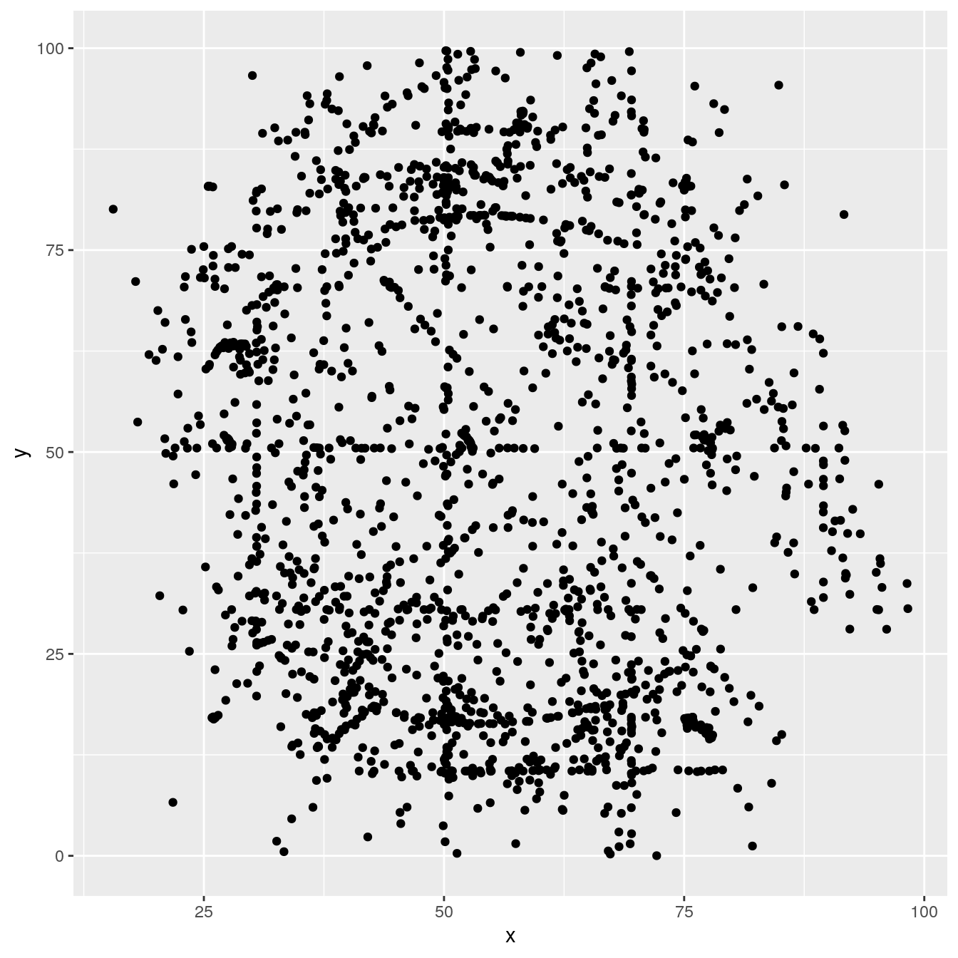
reuse the above command, and now colored by the dataset column
ggplot(ds_dozen, aes(x = x, y = y, colour = dataset)) +
  geom_point()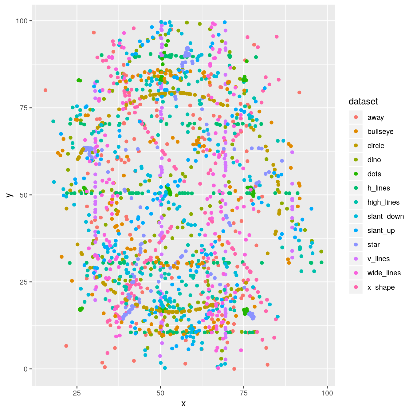
too many datasets are displayed, how can we plot only one at a time?
ds_dozen %>%
  filter(dataset == "away") %>%
  ggplot(aes(x = x, y = y)) +
  geom_point()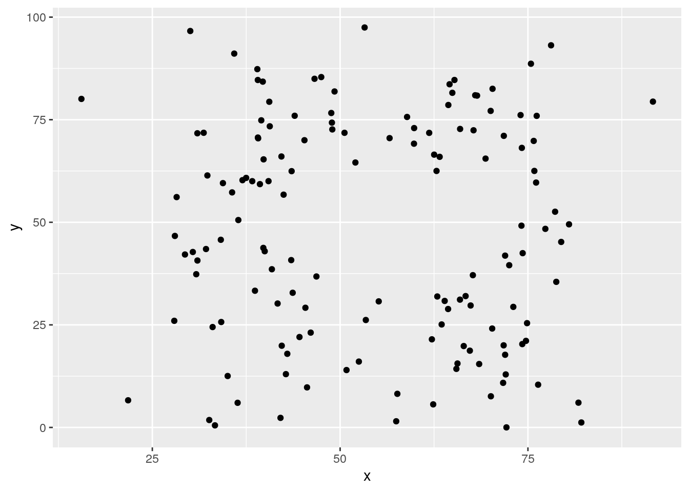
adjust the filtering step to plot two datasets?
Tip
R provides the inline instruction
%in% to test if there a match of the left operand in the right one (a vector most probably)
ds_dozen %>%
  filter(dataset %in% c("away", "dino")) %>%
  # alternative without %in% and using OR (|)
  #filter(dataset == "away" | dataset == "dino") %>%
  ggplot(aes(x = x, y = y, colour = dataset)) +
  geom_point()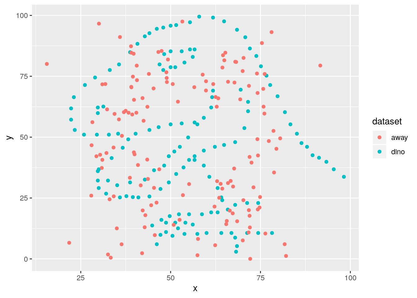
expand now by getting one dataset per facet
ds_dozen %>%
  filter(dataset %in% c("away", "dino")) %>%
  ggplot(aes(x = x, y = y, colour = dataset)) +
  geom_point() +
  facet_wrap(~ dataset)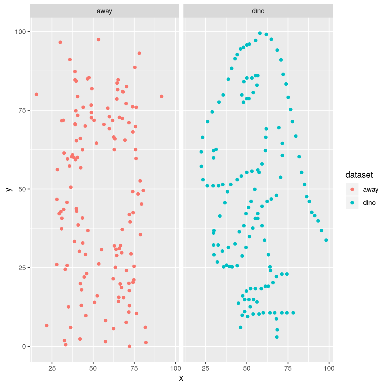
remove the filtering step to facet all datasets
ds_dozen %>%
  ggplot(aes(x = x, y = y, colour = dataset)) +
  geom_point() +
  facet_wrap(~ dataset, ncol = 3)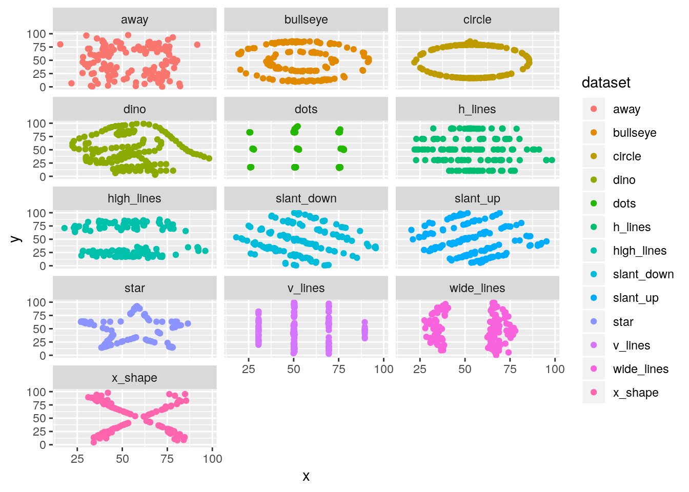
tweak the theme and use the theme_void and remove the legend
ggplot(ds_dozen, aes(x = x, y = y, colour = dataset)) +
  geom_point() +
  theme_void() +
  theme(legend.position = "none") +
  facet_wrap(~ dataset, ncol = 3)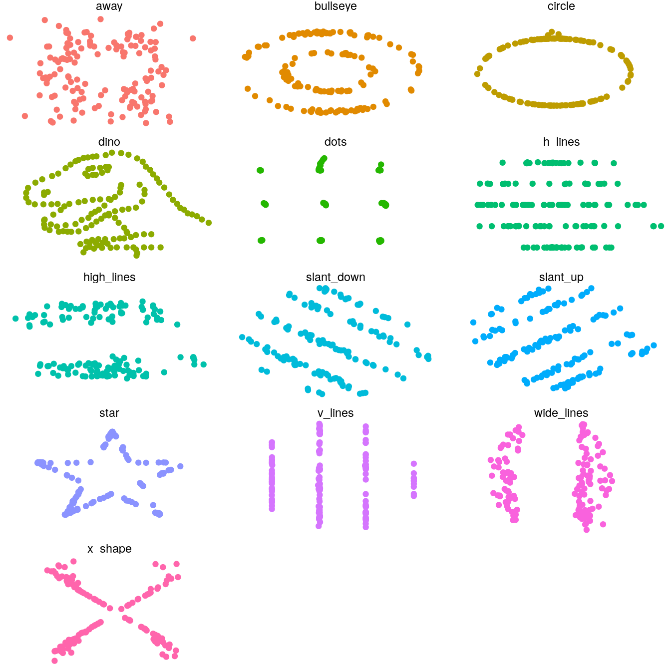
are the datasets actually that similar?
no ;) We were fooled by the summary stats
Tip
the R package gifski could be installed on your machine, makes the GIF creation faster.
install gganimate, its dependencies will be automatically installed.
install.packages("gganimate")use the dataset variable to the transition_states() argument layer
library(gganimate)

ds_dozen %>%
  ggplot(aes(x = x, y = y)) +
  geom_point() +
  # transition will be made using the dataset column
  transition_states(dataset, transition_length = 5, state_length = 2) +
  # for a firework effect!
  shadow_wake(wake_length = 0.05) +
  labs(title = "dataset: {closest_state}") +
  theme_void(14) +
  theme(legend.position = "none") -> ds_anim
# more frames to slow down the animation
ds_gif <- animate(ds_anim, nframes = 500, fps = 10)
ds_gif
anim_save(title_frame = TRUE, "./img/ds.gif")
visualized as small the differences in means for both coordinates
- need to zoom tremendously to see almost nothing. Accumule all states to better see the motions.
ds_dozen %>%
  group_by(dataset) %>%
  summarise_if(is.double, funs(mean = mean, sd = sd)) %>%
  ggplot(aes(x = x_mean, y = y_mean, colour = dataset)) +
  geom_point(size = 25, alpha = 0.6) +
  # zoom in like crazy
  coord_cartesian(xlim = c(54.25, 54.3), ylim = c(47.75, 47.9)) +
  # animate
  transition_states(dataset, transition_length = 5, state_length = 2) +
  # do not remove previous states to pile up dots
  shadow_mark() +
  labs(title = "dataset: {closest_state}") +
  theme_minimal(14) +
  theme(legend.position = "none") -> ds_mean_anim
ds_mean_gif <- animate(ds_mean_anim, nframes = 100, fps = 10)
ds_mean_gif
anim_save("img/ds_mean.gif")
Conclusion
never trust summary statistics alone; always visualize your data | Alberto Cairo
Authors
- Alberto Cairo, (creator)
- Justin Matejka
- George Fitzmaurice
- Lucy McGowan
from this post