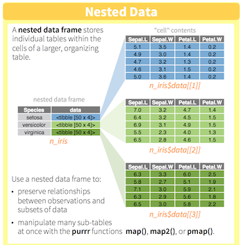
November 2019

Learning objectives

You will learn to:

  • use dplyr / purrr for efficient data manipulation
  • tidying multiple linear models using broom
  • managing related things together in one tibble
  • summarise findings in one ggplot using relevant aesthetics

guided practical

interactive session

Managing multiple models

list-column cheatsheet

reminder

Keep all analyse steps (cols) per group (rows) together

reminder

workflow from last time

mtcars %>%
  group_nest(cyl) %>%
  mutate(model = map(data, ~lm(mpg ~ wt, data = .x)),
         summary = map(model, summary),
         r_squared = map_dbl(summary, "r.squared"))
# A tibble: 3 x 5
    cyl data               model  summary    r_squared
  <dbl> <list>             <list> <list>         <dbl>
1     4 <tibble [11 × 10]> <lm>   <smmry.lm>     0.509
2     6 <tibble [7 × 10]>  <lm>   <smmry.lm>     0.465
3     8 <tibble [14 × 10]> <lm>   <smmry.lm>     0.423

Gapminder

gapminder is a fact tank

dataset

Hans Rosling

  • died 2 years ago
  • fundamentaly optimistic
  • great talk

Guided practical

explore gapminder

  • install the gapminder package
  • load gapminder and tidyverse packages
  • use the pipe %>% to pass gapminder to ggplot()
  • plot the life expectency (lifeExp in y) ~ year (x)
  • use geom_line()

warning!

  • mind the grouping!

Gapminder

global vs individual trend

library(gapminder)
gapminder %>%
  ggplot(aes(x = year, y = lifeExp, group = country)) +
  geom_line()

Keep related things together using list-columns

Keep related things together

group_nest()

One country example

Germany

from original tibble

gapminder %>%
  filter(country == "Germany") %>%
  select(-country, -continent, -pop)
# A tibble: 12 x 3
    year lifeExp gdpPercap
   <int>   <dbl>     <dbl>
 1  1952    67.5     7144.
 2  1957    69.1    10188.
 3  1962    70.3    12902.
 4  1967    70.8    14746.
 5  1972    71      18016.
 6  1977    72.5    20513.
 7  1982    73.8    22032.
 8  1987    74.8    24639.
 9  1992    76.1    26505.
10  1997    77.3    27789.
11  2002    78.7    30036.
12  2007    79.4    32170.

nested tibble

by_country %>%
  filter(country == "Germany")
# A tibble: 1 x 3
  continent country data             
  <fct>     <fct>   <list>           
1 Europe    Germany <tibble [12 × 5]>
by_country %>%
  filter(country == "Germany") %>%
  unnest(data) %>% 
  select(-country, -continent, -pop)
# A tibble: 12 x 4
    year lifeExp gdpPercap year1950
   <int>   <dbl>     <dbl>    <dbl>
 1  1952    67.5     7144.        2
 2  1957    69.1    10188.        7
 3  1962    70.3    12902.       12
 4  1967    70.8    14746.       17
 5  1972    71      18016.       22
 6  1977    72.5    20513.       27
 7  1982    73.8    22032.       32
 8  1987    74.8    24639.       37
 9  1992    76.1    26505.       42
10  1997    77.3    27789.       47
11  2002    78.7    30036.       52
12  2007    79.4    32170.       57

What happens in the DATA FRAME, stays in the data frame

Las Vegas principle, add linear models

  • using by_country
  • add a new column model with linear regressions of lifeExp on year1950
  • save as by_country_lm

ask yourself

  • if you see add column, do you use mutate or summarise?
  • dealing with a list-column (here the column data), do you need to use map?

Keep related things together

linear models

Explore a list column

  • count # rows per country using the data column
  • does any country have less data than others?

reminder

  • a list column is a list, you need to iterate through elements

Explore a list column

count how many rows per country

by_country_lm %>%
  mutate(n = map_int(data, nrow)) %>%
  select(country, n)
# A tibble: 142 x 2
   country                      n
   <fct>                    <int>
 1 Algeria                     12
 2 Angola                      12
 3 Benin                       12
 4 Botswana                    12
 5 Burkina Faso                12
 6 Burundi                     12
 7 Cameroon                    12
 8 Central African Republic    12
 9 Chad                        12
10 Comoros                     12
# … with 132 more rows
by_country_lm %>%
  mutate(n = map_int(data, nrow)) %>%
  distinct(n)
# A tibble: 1 x 1
      n
  <int>
1    12

Explore nested tibble

  • display the summary for the linear model of Rwanda
  • how do you interpret the \(r^2\) for this particular model?

reminder

  • filter() for the desired country
  • list column is a list
  • map() on the model column the function summary(), name it summary
  • extract the r.squared with map_dbl(summary, "r.squared")

Explore nested tibble

linear model for Rwanda

by_country_lm %>%
  filter(country == "Rwanda") %>%
  mutate(summary = map(model, summary),
         rsq = map_dbl(summary, "r.squared"))
# A tibble: 1 x 6
  continent country data              model  summary       rsq
  <fct>     <fct>   <list>            <list> <list>      <dbl>
1 Africa    Rwanda  <tibble [12 × 5]> <lm>   <smmry.lm> 0.0172

\(r^2\) is close to 0, linearity sounds broken

broom will cleanup lm elements into tibbles

broom cleanup

Tidying models

extract from nested lists

  • using by_country_lm, add 4 new columns:
    • glance, using the broom function on the model column
    • tidy, using the broom function on the model column
    • augment, using the broom function on the model column
    • rsq from the glance column
  • save as models
  • why extracting the \(r^2\) in the main tibble is useful?

reminder

  • use map when dealing with a list column
  • in map, shortcut with quotes (like "r.squared") extract the specified variable
  • map takes and returns a list. Use map_dbl() to coerce output to doubles

Tidying models

extract from nested lists

useful info

  • coefficients estimates:
    • slope
    • intercept
  • \(r^2\)
  • residuals
library(broom)
models <- by_country_lm %>%
  mutate(glance  = map(model, glance),
         tidy    = map(model, tidy),
         augment = map(model, augment),
         rsq     = map_dbl(glance, "r.squared"))
models
# A tibble: 142 x 8
   continent country      data     model  glance   tidy    augment      rsq
   <fct>     <fct>        <list>   <list> <list>   <list>  <list>     <dbl>
 1 Africa    Algeria      <tibble… <lm>   <tibble… <tibbl… <tibble … 0.985 
 2 Africa    Angola       <tibble… <lm>   <tibble… <tibbl… <tibble … 0.888 
 3 Africa    Benin        <tibble… <lm>   <tibble… <tibbl… <tibble … 0.967 
 4 Africa    Botswana     <tibble… <lm>   <tibble… <tibbl… <tibble … 0.0340
 5 Africa    Burkina Faso <tibble… <lm>   <tibble… <tibbl… <tibble … 0.919 
 6 Africa    Burundi      <tibble… <lm>   <tibble… <tibbl… <tibble … 0.766 
 7 Africa    Cameroon     <tibble… <lm>   <tibble… <tibbl… <tibble … 0.680 
 8 Africa    Central Afr… <tibble… <lm>   <tibble… <tibbl… <tibble … 0.493 
 9 Africa    Chad         <tibble… <lm>   <tibble… <tibbl… <tibble … 0.872 
10 Africa    Comoros      <tibble… <lm>   <tibble… <tibbl… <tibble … 0.997 
# … with 132 more rows

extracting \(r^2\) in main tibble

  • no need to unnest for sort / filtering.

Exploratory plots

plotting \(r^2\) for countries

  • plot country ~ rsq
  • reorder country levels by \(r^2\) (rsq): snake plot
  • color points per continent
  • which continent shows most of the low \(r^2\) values?

reminder

to reorder discrete values:

  • must be of data type factor
  • use the forcats package
  • fct_reorder() to reorder according to a continuous variable

Do linear models fit all countries?

snake plot

models %>%
  ggplot(aes(x = rsq, 
             y = fct_reorder(country,
                             rsq))) +
  geom_point(aes(colour = continent), 
             alpha = 0.5) +
  theme_classic(18) +
  theme(axis.text.y = element_blank(),
        axis.ticks.y = element_blank(),
        legend.position = c(0.25, 0.75)) +
   guides(color = guide_legend(
     override.aes = list(alpha = 1))) +
  labs(x = "r square",
       y = "Country") 

display the real data for countries with a low \(r^2\)

  • focus on non-linear trends
  • filter the 20 countries with the lowest \(r^2\)
  • unnest column data
  • plot lifeExp ~ year with lines
  • colour per continent
  • facet per country
  • same questions for the top 20 \(r^2\)

reminder

  • arrange(col) will sort according to col
  • top_n(x, col) not only sort col but return only x top entries
  • top_n(x, desc(col)) same but sort from lowest values

Exploratory plots

focus on non-linear trends

Exploratory plots

focus on linear trends

interpreting the linear model

regression

  • what represents the intercept?
    • using year1950?
    • using year?
    • justify Hadley choice
  • what represents the slope?

Germany, lifeExp ~ year1950

filter(models, country == "Germany") %>%
  unnest(tidy) %>%
  select(term, estimate, statistic)
# A tibble: 2 x 3
  term        estimate statistic
  <chr>          <dbl>     <dbl>
1 (Intercept)   67.1       282. 
2 year1950       0.214      30.7

Germany, lifeExp ~ year

# A tibble: 2 x 3
  term        estimate statistic
  <chr>          <dbl>     <dbl>
1 (Intercept) -350.        -25.4
2 year           0.214      30.7

Summarise on one plot

by Hadley Wickham

  • unnest coefficients (tidy column)
    • mind to keep the continent, country and rsq columns
  • put intercept and slope in their own columns
    • in wide format, only one value can be used.
    • discard unused columns.
  • plot slope ~ intercept (watch out the (Intercept) name which needs to be called between backsticks ‘`’)
  • colour per continent
  • size per \(r^2\) (use for scale_size_area() for lisibility)
  • add tendency with geom_smooth(method = "loess")

All in all

by Hadley Wickham

models %>%
  unnest(tidy) %>%
  select(continent, country, rsq, term, estimate) %>%
  pivot_wider(names_from = term, values_from = estimate) %>%
  ggplot(aes(x = `(Intercept)`, y = year1950)) +
  geom_point(aes(colour = continent, size = rsq)) +
  geom_smooth(se = FALSE, method = "loess") +
  scale_size_area() + labs(x = "Life expectancy (1950)", y = "Yearly improvement")

animation made easy

takes ~ 5 minutes due to easing

gganimate by Thomas Pedersen

library(gganimate)
gapminder %>%
  ggplot(aes(x = gdpPercap,
             y = lifeExp,
             size = pop, 
             color = continent)) +
  transition_time(year) +
  ease_aes("linear") +
  scale_size(range = c(2, 12)) +
  geom_point() +
  theme_bw(16) +
  labs(title = "Year: {frame_time}", 
       x = "GDP per capita", 
       y = "life expectancy") +
  scale_x_log10() -> p
animate(p)
anim_save("gapminder2.gif")

Before we stop

You learned to:

  • keep related things together:
    • input data
    • meaningful grouping ids
    • perform modelling
    • extract relevant model components
    • explore visually your findings

Acknowledgments

  • Hadley Wickham
  • Jennifer Bryan
  • David Robinson
  • Thomas Pedersen
  • Eric Koncina (iosp R package for slides)