Functional programming

November 2019

Learning objectives

You will learn to:

use a functional programming approach to simplify your code
pass functions as arguments to higher order functions
use purrr::map to replace for loops
use purrr::map together with nested tibbles

Reminder

vector & list

Atomic vectors

Each atomic vector contains only a single type of data

The type of each atom is the same
The size of each atom is 1 (single element)

Example

# Logical
c(TRUE, FALSE, TRUE)

[1]  TRUE FALSE  TRUE

# double
c(1, 5, 7)

[1] 1 5 7

# character
c("character", "sequence")

[1] "character" "sequence"

Reminder

vector & list

Coercion

Is the conversion between types
Can be
- explicit (using as.*() functions)
- implicit

Explicit

v_example <- c(1, 3, 7)
str(as.character(v_example))

 chr [1:3] "1" "3" "7"

Implicit

v_example <- c(1, 3)
str(v_example)

 num [1:2] 1 3

str(c(v_example, "seven"))

 chr [1:3] "1" "3" "seven"

Adapted from the tutorial of Jennifer Bryan

Reminder

vector & list

Lists

are vectors which are not atomic.
- Elements can be of different types
- The length of each element (atom) might be greater than 1.

Example

my_list <- list(1, 3, "seven")
str(my_list)

List of 3
 $ : num 1
 $ : num 3
 $ : chr "seven"

is.vector(my_list)

[1] TRUE

is.atomic(my_list)

[1] FALSE

Adapted from the tutorial of Jennifer Bryan

Reminder

functions

Declared function

my_function <- function(my_argument) {
  my_argument + 1
}

is defined in the global environment

ls()

[1] "my_function"

ls.str()

my_function : function (my_argument)

is reusable
```
my_function(2)
```
```
[1] 3
```

Anonymous functions

Are not stored in an object and are used “on the fly”

(function(x) { x + 1 })(2)

[1] 3

Does not alter the global environment

ls()

[1] "my_function"

# remove the previous my_function to convince you
rm(my_function)
(function(x) { x + 1 })(2)

[1] 3

ls()

character(0)

Purrr

functional programming

Overview

purrr enhances R’s functional programming toolkit by providing a complete and consistent set of tools for working with functions and vectors (purrr overview on github page)

functional programming is a programming paradigm – a style of building the structure and elements of computer programs – that treats computation as the evaluation of mathematical functions and avoids changing-state and mutable data Wikipedia

Purrr

focuses on functions

functional programming features

pass functions as arguments to other functions
code that does not change state (a same call should yield the same result)

Use it for iterations

FOR EACH x DO f

Iteration

the LEGO example

Consider a hypothetic `put_on` function

put_on(x, antenna)

legos

antenna

lego with antenna

Iteration

the LEGO example

Illustration

legos

antenna

legos with antennas

LEGO pictures from Jennifer Bryan

for loop approach

out <- vector("list", length(legos))
for (i in seq_along(legos)) {
  out[[i]] <- put_on(legos[[i]], antenna)
}
out

functional programming approach

antennate <- function(x) put_on(x, antenna)
map(legos, antennate)

Your turn

Reminder

a data frame is a list
```
is.list(mtcars)
```
```
[1] TRUE
```
Each column represents an element of the list i.e. a data frame is a list of columns

Exercise

Calculate the mean of each column of the mtcars dataset.

Your turn

03:00

Using `purrr::map()`

map(mtcars, mean) %>%
  str()

List of 11
 $ mpg : num 20.1
 $ cyl : num 6.19
 $ disp: num 231
 $ hp  : num 147
 $ drat: num 3.6
 $ wt  : num 3.22
 $ qsec: num 17.8
 $ vs  : num 0.438
 $ am  : num 0.406
 $ gear: num 3.69
 $ carb: num 2.81

`for` loops

means <- vector("list", ncol(mtcars))
for (i in seq_along(mtcars)) {
  means[i] <- mean(mtcars[[i]])
}
# need to manually add names
names(means) <- names(mtcars)
means %>%
  str()

List of 11
 $ mpg : num 20.1
 $ cyl : num 6.19
 $ disp: num 231
 $ hp  : num 147
 $ drat: num 3.6
 $ wt  : num 3.22
 $ qsec: num 17.8
 $ vs  : num 0.438
 $ am  : num 0.406
 $ gear: num 3.69
 $ carb: num 2.81

For loops are fine

growing

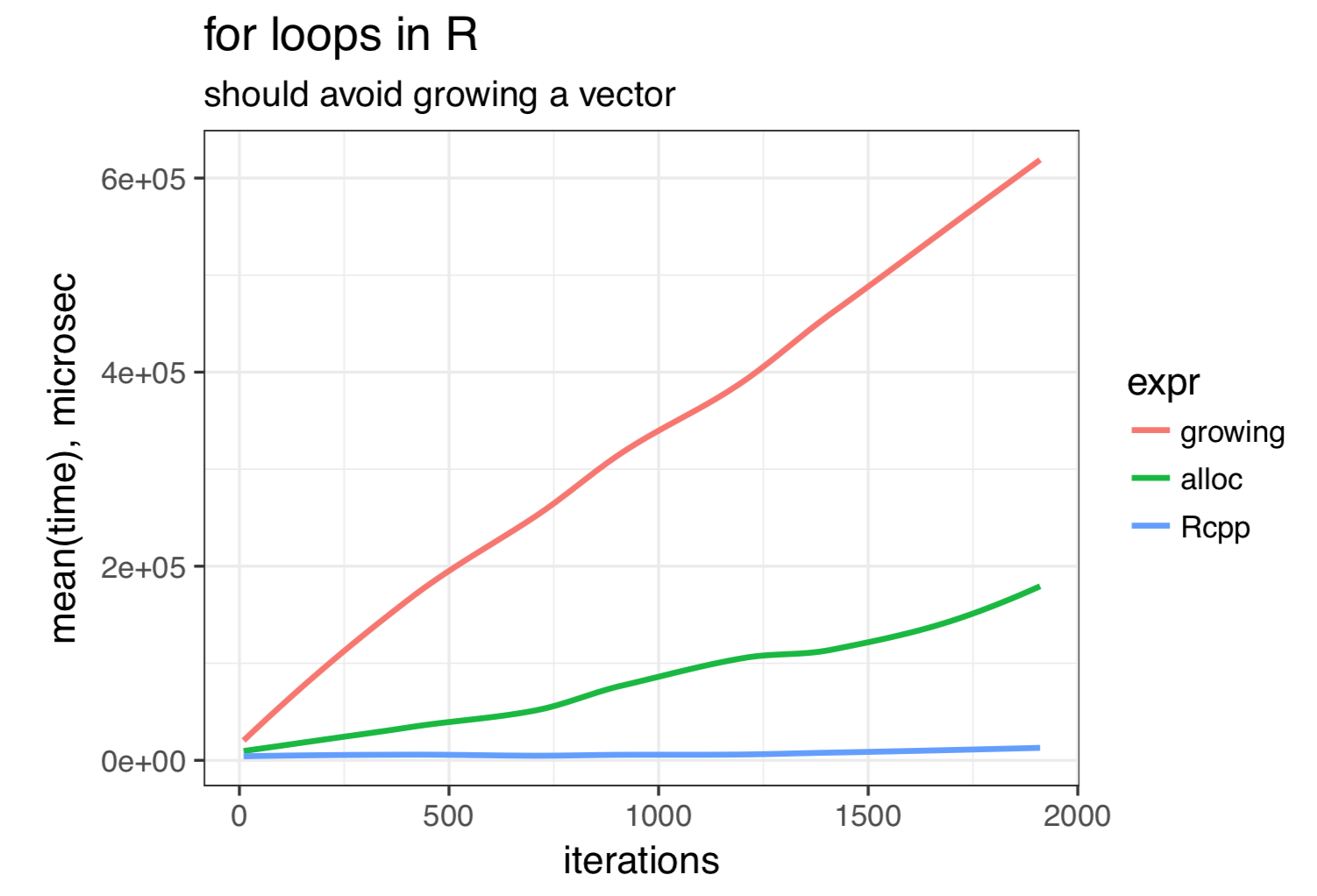
for_loop <- function(x) {
  res <- c()
  for (i in seq_len(x)) {
    res[i] <- i
  }
}

alloc

for_loop <- function(x) {
  res <- vector(mode = "integer", 
                length = x)
  for (i in seq_len(x)) {
    res[i] <- i
  }
}

Rcpp

library(Rcpp)
cppFunction("NumericVector rcpp(int x) {
  NumericVector res(x);
  for (int i=0; i < x; i++) {
    res[i] = i;
  }
}")

Iteration

the LEGO example

Illustration

legos

antenna

map(legos, antennate)

LEGO pictures from Jennifer Bryan

`purrr::map()` is type stable

applies a function to each element of a list / vector
returns a list
map(YOUR_LIST, YOUR_FUNCTION)

`base::apply()` vs `purrr::map()`

Warning

apply() family of function is inconsistent and some members are not type stable.
Exception: lapply()
apply() family still useful to avoid dependencies (package development)

The apply family of functions

function	call	input	output
`apply()`	`apply(X, MARGIN, FUN, ...)`	array	vector or array or list
`lapply()`	`lapply(X, FUN, ...)`	list	list
`sapply()`	`sapply(X, FUN, ...)`	list	vector or array or list
`vapply()`	`vapply(X, FUN, FUN.VALUE, ...)`	list	specified

`base::apply()` vs `purrr::map()`

Example

`apply()`

apply(mtcars, 2, mean) %>% str()

 Named num [1:11] 20.09 6.19 230.72 146.69 3.6 ...
 - attr(*, "names")= chr [1:11] "mpg" "cyl" "disp" "hp" ...

`lapply()`

lapply(mtcars, mean) %>% str()

List of 11
 $ mpg : num 20.1
 $ cyl : num 6.19
 $ disp: num 231
 $ hp  : num 147
 $ drat: num 3.6
 $ wt  : num 3.22
 $ qsec: num 17.8
 $ vs  : num 0.438
 $ am  : num 0.406
 $ gear: num 3.69
 $ carb: num 2.81

`base::apply()` vs `purrr::map()`

Example data

Let’s create the following tibbles:

tib_1 <- tibble(a = 1:3, b = 4:6, c = 7:9)
tib_2 <- tibble(a = 1:3, b = 4:6, c = 11:13)

`troublemaker` function

troublemaker <- function(x) {
  if (any(x > 10)) return(NULL)
  sum(x)
}

troublemaker_chr <- function(x) {
  if (any(x > 10)) return(as.character(sum(x)))
  sum(x)
}

Define some troublemaker functions:

returns the sum of the input vector
if any number is greater than 10:
- troublemaker() returns NULL
- troublemaker_chr() coerces the sum to a character

`base::apply()` vs `purrr::map()`

`troublemaker` example

troublemaker(1:3)

[1] 6

troublemaker(11:13)

NULL

troublemaker_chr(1:3)

[1] 6

troublemaker_chr(11:13)

[1] "36"

`lapply()`

lapply(tib_1, troublemaker) %>% str()

List of 3
 $ a: int 6
 $ b: int 15
 $ c: int 24

lapply(tib_2, troublemaker) %>% str()

List of 3
 $ a: int 6
 $ b: int 15
 $ c: NULL

lapply(tib_2, troublemaker_chr) %>% str()

List of 3
 $ a: int 6
 $ b: int 15
 $ c: chr "36"

`map()`

map(tib_1, troublemaker) %>% str()

List of 3
 $ a: int 6
 $ b: int 15
 $ c: int 24

map(tib_2, troublemaker) %>% str()

List of 3
 $ a: int 6
 $ b: int 15
 $ c: NULL

map(tib_2, troublemaker_chr) %>% str()

List of 3
 $ a: int 6
 $ b: int 15
 $ c: chr "36"

`base::apply()` vs `purrr::map()`

`apply()`

apply(tib_1, 2, troublemaker) %>% str()

 Named int [1:3] 6 15 24
 - attr(*, "names")= chr [1:3] "a" "b" "c"

apply(tib_2, 2, troublemaker) %>% str()

List of 3
 $ a: int 6
 $ b: int 15
 $ c: NULL

apply(tib_2, 2, troublemaker_chr) %>% str()

 Named chr [1:3] "6" "15" "36"
 - attr(*, "names")= chr [1:3] "a" "b" "c"

Warning

In addition to the confusing margin argument, apply() simplifies the output value: read the help ?apply.

If each call to FUN returns a vector of length n, then apply returns an array of dimension c(n, dim(X)[MARGIN]) if n > 1. If n equals 1, apply returns a vector if MARGIN has length 1 and an array of dimension dim(X)[MARGIN] otherwise. If n is 0, the result has length 0 but not necessarily the ‘correct’ dimension.
If the calls to FUN return vectors of different lengths, apply returns a list of length prod(dim(X)[MARGIN]) with dim set to MARGIN if this has length greater than one.
In all cases the result is coerced by as.vector to one of the basic vector types before the dimensions are set, so that (for example) factor results will be coerced to a character array. value definition in ?apply

`purrr::map()`

`map()` variants

purrr provides variants coercing the output to the desired output. Generates an error if the mapped function produces an unexpected output.

`map_dbl()`

map_dbl(tib_1, troublemaker) %>%
  str()

 Named num [1:3] 6 15 24
 - attr(*, "names")= chr [1:3] "a" "b" "c"

map_dbl(tib_2, troublemaker) %>%
  str()

Result 3 must be a single double, not NULL of length 0

map_dbl(tib_2, troublemaker_chr) %>%
  str()

Error: Can't coerce element 3 from a character to a double

`base::apply()` vs `purrr::map()`

The `purrr::map()` family of functions

are designed to be consistent
map() is the general function and close to base::lapply()
map() introduces shortcuts (absent in lapply())
variants to specify the type of vectorized output:
- map_lgl()
- map_int()
- map_dbl()
- map_chr()
- map_df()

`purrr::map()` example

example dataset: generate a list of data frames

Let’s split the mtcars dataset by each value of cylinder

spl_mtcars <- group_split(mtcars, mtcars$cyl)
str(spl_mtcars, max.level = 1)

List of 3
 $ :Classes 'tbl_df', 'tbl' and 'data.frame':   11 obs. of  12 variables:
 $ :Classes 'tbl_df', 'tbl' and 'data.frame':   7 obs. of  12 variables:
 $ :Classes 'tbl_df', 'tbl' and 'data.frame':   14 obs. of  12 variables:
 - attr(*, "ptype")=Classes 'tbl_df', 'tbl' and 'data.frame':   0 obs. of  12 variables:
  ..- attr(*, "groups")=Classes 'tbl_df', 'tbl' and 'data.frame':   3 obs. of  2 variables:
  .. ..- attr(*, ".drop")= logi TRUE

On each element (dataframe) of the list, we would like to:
- fit a linear model (miles per gallon explained by the weight)
- extract the \(r^2\) value

From R for Data Science

Reminder

Fit a linear model

Using the mtcars dataset we can fit a linear model to explain the miles per gallon (mpg) by the weight (wt) using:

lm(mpg ~ wt, data = mtcars)

Call:
lm(formula = mpg ~ wt, data = mtcars)

Coefficients:
(Intercept)           wt  
     37.285       -5.344

Reminder, `lm` outputs complex objects

Summarise a linear model

base::summary() summaries the model:

lm(mpg ~ wt, data = mtcars) %>%
  summary()

Call:
lm(formula = mpg ~ wt, data = mtcars)

Residuals:
    Min      1Q  Median      3Q     Max 
-4.5432 -2.3647 -0.1252  1.4096  6.8727 

Coefficients:
            Estimate Std. Error t value Pr(>|t|)    
(Intercept)  37.2851     1.8776  19.858  < 2e-16 ***
wt           -5.3445     0.5591  -9.559 1.29e-10 ***
---
Signif. codes:  0 '***' 0.001 '**' 0.01 '*' 0.05 '.' 0.1 ' ' 1

Residual standard error: 3.046 on 30 degrees of freedom
Multiple R-squared:  0.7528,    Adjusted R-squared:  0.7446 
F-statistic: 91.38 on 1 and 30 DF,  p-value: 1.294e-10

`purrr::map()` example

05:00

1 - for each cyl group

So for the 3 cyl groups:

fit a linear model (miles per gallon explained by the weight)
- the equation is then: \(mpg = \beta_0 + \beta_1 \times wt\),
- formula in R: mpg ~ wt

1 - map the linear model

map(YOUR_LIST, YOUR_FUNCTION)
YOUR_LIST = spl_mtcars
YOUR_FUNCTION can be an anonymous function (declared on the fly)

map(spl_mtcars, function(x) lm(mpg ~ wt, data = x))

[[1]]

Call:
lm(formula = mpg ~ wt, data = x)

Coefficients:
(Intercept)           wt  
     39.571       -5.647  


[[2]]

Call:
lm(formula = mpg ~ wt, data = x)

Coefficients:
(Intercept)           wt  
      28.41        -2.78  


[[3]]

Call:
lm(formula = mpg ~ wt, data = x)

Coefficients:
(Intercept)           wt  
     23.868       -2.192

`purrr::map()` example

map(spl_mtcars,
    function(x) lm(mpg ~ wt, data = x))

[[1]]

Call:
lm(formula = mpg ~ wt, data = x)

Coefficients:
(Intercept)           wt  
     39.571       -5.647  


[[2]]

Call:
lm(formula = mpg ~ wt, data = x)

Coefficients:
(Intercept)           wt  
      28.41        -2.78  


[[3]]

Call:
lm(formula = mpg ~ wt, data = x)

Coefficients:
(Intercept)           wt  
     23.868       -2.192

Reminder

`base::summary()` generates a list

lm(mpg ~ wt, data = mtcars) %>%
  summary() %>%
  str(max.level = 1, give.attr = FALSE)

List of 11
 $ call         : language lm(formula = mpg ~ wt, data = mtcars)
 $ terms        :Classes 'terms', 'formula'  language mpg ~ wt
 $ residuals    : Named num [1:32] -2.28 -0.92 -2.09 1.3 -0.2 ...
 $ coefficients : num [1:2, 1:4] 37.285 -5.344 1.878 0.559 19.858 ...
 $ aliased      : Named logi [1:2] FALSE FALSE
 $ sigma        : num 3.05
 $ df           : int [1:3] 2 30 2
 $ r.squared    : num 0.753
 $ adj.r.squared: num 0.745
 $ fstatistic   : Named num [1:3] 91.4 1 30
 $ cov.unscaled : num [1:2, 1:2] 0.38 -0.1084 -0.1084 0.0337

Extract \(r^2\)

fit_summary <- summary(lm(mpg ~ wt, data = mtcars))
fit_summary$r.squared

[1] 0.7528328

`purrr::map()` example

2 - extract \(r^2\)

map uses a list as an argument and returns a list
we can map a new function on the output of the previous call
works well in a pipeline (using %>%)

spl_mtcars %>% 
  map(function(x) lm(mpg ~ wt, data = x)) %>%
  map(summary) %>%
  map(function(x) x$r.squared)

[[1]]
[1] 0.5086326

[[2]]
[1] 0.4645102

[[3]]
[1] 0.4229655

Tip

The code above can be simplified using shortcuts provided by purrr

`purrr::map()` shortcuts

Anonymous functions

One sided formula create anonymous functions:
- define the function using ~
- use the placeholder .x to refer to the current list element (.x represents the argument of the anonymous function)
```
map(YOUR_LIST, function(x) lm(mpg ~ wt, data = x))

# is equivalent to:

map(YOUR_LIST, ~ lm(mpg ~ wt, data = .x))
```

Initial code

spl_mtcars %>% 
  map(function(x) lm(mpg ~ wt, data = x)) %>%
  map(summary) %>%
  map(function(x) x$r.squared)

With anon. function shortcuts

spl_mtcars %>% 
  map(~lm(mpg ~ wt, data = .x)) %>%
  map(summary) %>%
  map(~.x$r.squared)

`purrr::map()` shortcuts

Named components

Use a string to extract named components

map(spl_mtcars, "mpg")

[[1]]
 [1] 22.8 24.4 22.8 32.4 30.4 33.9 21.5 27.3 26.0 30.4 21.4

[[2]]
[1] 21.0 21.0 21.4 18.1 19.2 17.8 19.7

[[3]]
 [1] 18.7 14.3 16.4 17.3 15.2 10.4 10.4 14.7 15.5 15.2 13.3 19.2 15.8 15.0

Use a number to extract by index

map(spl_mtcars, 1)

[[1]]
 [1] 22.8 24.4 22.8 32.4 30.4 33.9 21.5 27.3 26.0 30.4 21.4

[[2]]
[1] 21.0 21.0 21.4 18.1 19.2 17.8 19.7

[[3]]
 [1] 18.7 14.3 16.4 17.3 15.2 10.4 10.4 14.7 15.5 15.2 13.3 19.2 15.8 15.0

`purrr::map()` shortcuts

Initial code

spl_mtcars %>% 
  map(function(x) lm(mpg ~ wt, data = x)) %>%
  map(summary) %>%
  map(function(x) x$r.squared)

[[1]]
[1] 0.5086326

[[2]]
[1] 0.4645102

[[3]]
[1] 0.4229655

Using shortcuts 1

spl_mtcars %>% 
  map(~lm(mpg ~ wt, data = .x)) %>%
  map(summary) %>%
  map(~.x$r.squared)

[[1]]
[1] 0.5086326

[[2]]
[1] 0.4645102

[[3]]
[1] 0.4229655

Using shortcuts 2

spl_mtcars %>% 
  map(~lm(mpg ~ wt, data = .x)) %>%
  map(summary) %>%
  map("r.squared")

[[1]]
[1] 0.5086326

[[2]]
[1] 0.4645102

[[3]]
[1] 0.4229655

`purrr::map_*()` variants

using `map()`

spl_mtcars %>% 
  map(~lm(mpg ~ wt, data = .x)) %>%
  map(summary) %>%
  map("r.squared") %>% 
  str()

List of 3
 $ : num 0.509
 $ : num 0.465
 $ : num 0.423

using `map_dbl()`

spl_mtcars %>% 
  map(~lm(mpg ~ wt, data = .x)) %>%
  map(summary) %>%
  map_dbl("r.squared") %>% 
  str()

 num [1:3] 0.509 0.465 0.423

`purrr::map()` and mutliple arguments

Additional function arguments

You can use purrr::map() shortcuts to pass additional (constant) arguments

Initial example

antennate <- function(x) put_on(x, antenna)
map(legos, antennate)

Using anonymous function

map(legos, ~ put_on(.x, antenna))

Shortcut for additional arguments

map(legos, put_on, antenna)

Iterating on 2 lists

`map()` for a single list

map(legos, antennate)

`map2()` for two lists

enhair <- function(x, y) put_on(x, y)
map2(legos, hairs, enhair)

Iterating on several lists

pmap(.l, .f, ...)

Supply the different lists as a list of list (.l)
Placeholder in the anonymous function is: ..1, ..2, ..3, …

`pmap()` example

my_list <- list(
  list(1, 5, 7),
  list(6, 10, 9),
  list(1, 2, 0.5)
     )

pmap(my_list,
     function(a, b, c) {seq(from = a, to = b, by = c)}
     ) %>%
  str()

List of 3
 $ : num [1:6] 1 2 3 4 5 6
 $ : num [1:3] 5 7 9
 $ : num [1:5] 7 7.5 8 8.5 9

pmap(my_list, ~seq(from = ..1, to = ..2, by = ..3)) %>%
  str()

List of 3
 $ : num [1:6] 1 2 3 4 5 6
 $ : num [1:3] 5 7 9
 $ : num [1:5] 7 7.5 8 8.5 9

Mapping a function for its side-effects

side-effects

A function might be called for its side-effects:

output on screen
save files to disk

Use the `walk` family of function

walk(), walk2(), pwalk()
returns the input list
can be used in a pipeline (%>%)

The tidyverse focuses on data frames

pros

easy
works with dplyr
nicely structured

cons

same length requirement
atomic vectors

solution

Use lists! But inside the tidyverse
- tibble introduces list-columns
- works with dplyr
- groups are respected
- easily created with group_nest()
- perfect input for purrr::map()

Lists as a column in a tibble

Example

tibble(numbers = 1:8,
       my_list = list(a = c("a", "b"), b = 2.56, 
                      c = c("a", "b"), d = rep(TRUE, 4),
                      d = 2:3, e = 4:6, f = "Z", g = 1:4))

# A tibble: 8 x 2
  numbers my_list     
    <int> <named list>
1       1 <chr [2]>   
2       2 <dbl [1]>   
3       3 <chr [2]>   
4       4 <lgl [4]>   
5       5 <int [2]>   
6       6 <int [3]>   
7       7 <chr [1]>   
8       8 <int [4]>

Example

Rewriting our previous example

Nesting the tibble by cylinder

mtcars %>%
  group_nest(cyl)

# A tibble: 3 x 2
    cyl data              
  <dbl> <list>            
1     4 <tibble [11 × 10]>
2     6 <tibble [7 × 10]> 
3     8 <tibble [14 × 10]>

Example

Rewriting our previous example

Use mutate and map

mtcars %>%
  group_nest(cyl) %>%
  mutate(model = map(data, ~lm(mpg ~ wt, data = .x)),
         summary = map(model, summary),
         r_squared = map_dbl(summary, "r.squared"))

# A tibble: 3 x 5
    cyl data               model  summary    r_squared
  <dbl> <list>             <list> <list>         <dbl>
1     4 <tibble [11 × 10]> <lm>   <smmry.lm>     0.509
2     6 <tibble [7 × 10]>  <lm>   <smmry.lm>     0.465
3     8 <tibble [14 × 10]> <lm>   <smmry.lm>     0.423

very powerful
data rectangle
next lecture will show you how dplyr, tidyr, tibble, purrr and broom nicely work together

Purrr

Pure functions

Make your pure #rstats functions purr with purrr, a new package for functional programming: http://t.co/91Efuz0txk
— Hadley Wickham (@hadleywickham) 29 septembre 2015

A function is called “pure” if all its inputs are declared as inputs - none of them are hidden - and likewise all its outputs are declared as outputs Kris Jenkins

“Purify” functions

Pure functions

Impure function

has hidden inputs or outputs
hidden inputs and/or outputs are called side-effects

start <- 10

impure <- function(x) {
  print(start)
  x + start
}

result <- impure(2)

[1] 10

result

[1] 12

Pure function

no hidden inputs and/or outputs

pure <- function(x, start) {
  x + start
}

result <- pure(2, start)
result

[1] 12

“Purify” functions

Example

Even log() has side-effects
Use purrr::safely() to catch every output

Impure `log()`

(res <- log(10))

[1] 2.302585

res <- log("a")

Error in log("a"): non-numeric argument to mathematical function

res

[1] 2.302585

Purified `log()`

safe_log <- purrr::safely(log)
(res <- safe_log(10))

$result
[1] 2.302585

$error
NULL

res <- safe_log("a")
res

$result
NULL

$error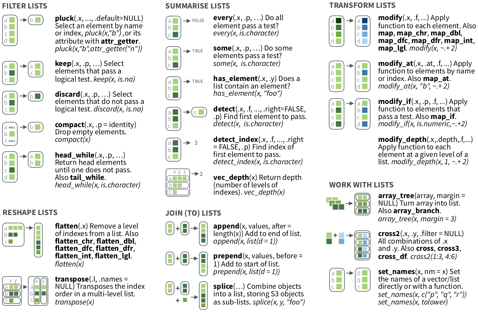
<simpleError in .Primitive("log")(x, base): non-numeric argument to mathematical function>

Many more verbs

Cheatsheet

Have a look at the purrr cheatsheet

Work with lists (Cheatsheet)

Wrap up

`map()` or `walk()`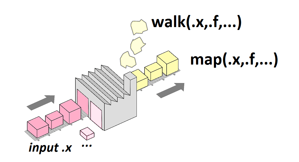

`map2()` or `walk2()`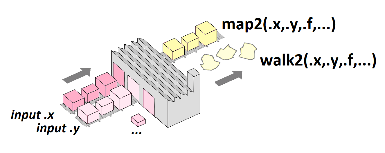

`pmap()`

Pictures from Lise Vaudor’s blog

Don’t forget vectorisation

Warning

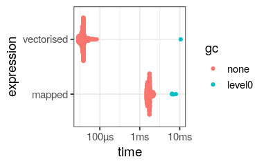
Don’t overmap functions!
Use map only if required (non vectorised function)

example

nums <- sample(1:10,
               size = 1000,
               replace = TRUE) 

log_vec <- log(nums)
log_map <- map_dbl(nums, log)

identical(log_vec, log_map)

[1] TRUE

benchmark

bench::mark(
  vectorised = log(nums),
  mapped = map_dbl(nums, log)) %>%
  autoplot()

Before we stop

Acknowledgments

Jennifer Bryan (LEGO pictures, courtesy CC licence)
Hadley Wickham
Lise Vaudor
Eric Koncina (iosp R package for slides) & content
Ian Lyttle

Learning objectives

You will learn to:

Reminder

vector & list

Atomic vectors

Example

Reminder

vector & list

Coercion

Explicit

Implicit

Reminder

vector & list

Lists

Example

Reminder

functions

Declared function

Anonymous functions

Purrr

Purrr

functional programming

Overview

Purrr

focuses on functions

functional programming features

Use it for iterations

Iteration

the LEGO example

Consider a hypothetic put_on function

Iteration

the LEGO example

Illustration

for loop approach

functional programming approach

Your turn

Reminder

Exercise

Your turn

Using purrr::map()

for loops

For loops are fine

growing

alloc

Rcpp

Iteration

the LEGO example

Illustration

purrr::map() is type stable

base::apply() vs purrr::map()

Warning

The apply family of functions

base::apply() vs purrr::map()

Example

apply()

lapply()

base::apply() vs purrr::map()

Example data

troublemaker function

base::apply() vs purrr::map()

troublemaker example

lapply()

map()

base::apply() vs purrr::map()

apply()

Warning

purrr::map()

map() variants

map_dbl()

base::apply() vs purrr::map()

The purrr::map() family of functions

purrr::map() example

example dataset: generate a list of data frames

Reminder

Fit a linear model

Reminder, lm outputs complex objects

Summarise a linear model

purrr::map() example

1 - for each cyl group

1 - map the linear model

Consider a hypothetic `put_on` function

Using `purrr::map()`

`for` loops

`purrr::map()` is type stable

`base::apply()` vs `purrr::map()`

`base::apply()` vs `purrr::map()`

`apply()`

`lapply()`

`base::apply()` vs `purrr::map()`

`troublemaker` function

`base::apply()` vs `purrr::map()`

`troublemaker` example

`lapply()`

`map()`

`base::apply()` vs `purrr::map()`

`apply()`

`purrr::map()`

`map()` variants

`map_dbl()`

`base::apply()` vs `purrr::map()`

The `purrr::map()` family of functions

`purrr::map()` example

Reminder, `lm` outputs complex objects

`purrr::map()` example

`purrr::map()` example

`base::summary()` generates a list

`purrr::map()` example

`purrr::map()` shortcuts

`purrr::map()` shortcuts

`purrr::map()` shortcuts

`purrr::map_*()` variants

using `map()`

using `map_dbl()`

`purrr::map()` and mutliple arguments

`map()` for a single list

`map2()` for two lists

`pmap()` example

Use the `walk` family of function

Impure `log()`

Purified `log()`

`map()` or `walk()`

`map2()` or `walk2()`

`pmap()`