Regression

November 2019

Learning objectives

You will learn:

what is a model?
model categories depending on data
perform linear models
assess linear models
know when you should move beyond linearity

Reading

An Introduction to Statistical Learning by James, Witten, Hastie & Tibshirani

Regression / Classification

when the response is continuous

Classification

when the response is categorical

Regression

assumptions

response must be a continous variables
modelling of increasing complexity:
- linear
- generalized linear
- polynomial
- non-linear
- non-parametric, smoothing such as splines

global form of modelling

\[Y = f(X) + \epsilon\]

where:

$Y$ is the response
$f$ represents the systematic information that $X$ provides about $Y$.
$\epsilon$ is the random error term
- independent from $X$
- has a mean of zero.

$f$ and residuals

simulated data ( in blue) and 30 observations

Income could be predicted by years of educations

Residuals

individual observation errors
have mean $\approx$ zero.
diff real $f$ to model $\hat{f}$
here as vertical black lines

$f$ is usually never known, use hats (^) for approximations

build models that approximate $f$ predicting response when error averages zero:

\[\hat{Y} = \hat{f}(X)\]

Prediction

when $\hat{f}$ is a black box, precision of $\hat{Y}$ matters

Goal is to minimized: \[E(Y - \hat{Y})^2 = [f(X) - \hat{f}(X)]^2 + Var(\epsilon)\]
where $Var(\epsilon)$ is the irreductible error.

Inference

when estimating $\hat{f}$ as accurately as possible matters

when several predictors exist, which are the important ones?
what is the shape of f?

How to estimate $f$?

training / test sets

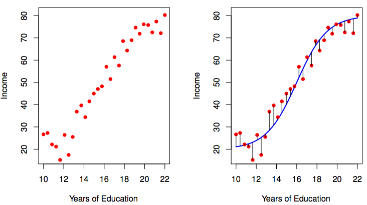
To estimate $f$, one usually uses a limited number of observations.

Here for example:
- 30 observations were used to obtain $\hat{f}$ (using a natural spline).
- Using 30 different observations, $\hat{f}$ would be different.
This initial dataset is called training data.
A good model will perform well on a test data

this purple $\hat{f}$ is different from the true blue $f$

How to estimate f?

parametric / non-parametric

parametric

involves 2 steps
- assumption on the shape of $f$ (linear, quadratic etc.)
- fit the model to the training data $\Rightarrow$ coefficients

non-parametric

implies some kind of smoothing.
- More flexible since no assumption on $f$ shape.
- Choosing the degree is smoothing is not easy and could lead to overfitting

Pushing too far non-parametric regressions

risk of overfitting

perfect match to the training data
no residuals!
makes model useless for test data

Linear model, parametric

The first step of the parametric approach is done:

f is linear

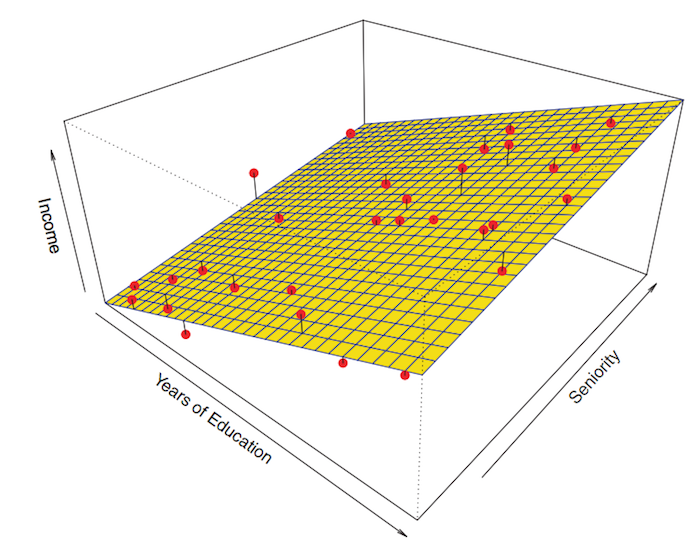
The general formula for p parameters gives p coefficients (slope) and $\beta_0$ the intercept

\[f(X) = \beta_0 + \beta_1 \times X_1 + \beta_2 \times X_2 + \ldots + \beta_p \times X_p\]

The model tries to minimize the reducible error, i. e the Sum of Squares of residuals

irreducible error, $\epsilon$

because unmeasured co-variables
because unmeasured variation (discrete times)
provide an upper bound on the accuracy of prediction

the usual method is the ordinary least squares

source: Logan M.

Minimized Residual Sum of Squares

RSS

In the regression $sales = \beta_0 + \beta_1 \times TV$

\[RSS = \sum_{i=1}^n{(y_i - \hat{y_i})^2}\]

Sum of squares

from lecture 8

demonstrated as a dynamic linear regression

Second step: coefficients estimations

empirical

graphically

estimate the intercept and the slope, $\Rightarrow$ is the response increase for 1 unit of the predictor.

advertising dataset

solution

intercept $\approx$ 7
slope $\approx$ 2 / 50 = 0.04

Second step: coefficients estimations

R

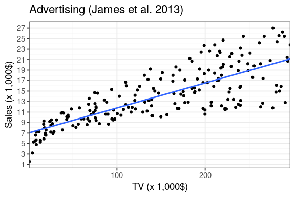
read_csv("data/Advertising.csv",
         col_types = cols()) %>%
  lm(Sales ~ TV, data = .) %>%
  summary()

Call:
lm(formula = Sales ~ TV, data = .)

Residuals:
    Min      1Q  Median      3Q     Max 
-8.3860 -1.9545 -0.1913  2.0671  7.2124 

Coefficients:
            Estimate Std. Error t value Pr(>|t|)    
(Intercept) 7.032594   0.457843   15.36   <2e-16 ***
TV          0.047537   0.002691   17.67   <2e-16 ***
---
Signif. codes:  0 '***' 0.001 '**' 0.01 '*' 0.05 '.' 0.1 ' ' 1

Residual standard error: 3.259 on 198 degrees of freedom
Multiple R-squared:  0.6119,    Adjusted R-squared:  0.6099 
F-statistic: 312.1 on 1 and 198 DF,  p-value: < 2.2e-16

Standard Errors of coefficients

RSE

\[RSE = \sqrt{\frac{RSS}{n - 2}}\] why $-2$ ?

SE

\[SE(\hat{\beta_{1}})^2 = \frac{RSE}{\sum_{i=1}^n(x_i - \hat{x})^2}\]

with this standard error, one per coefficient, we can compute confidence intervals

Standard Errors of coefficients: confidence intervals

read_csv("data/Advertising.csv") %>%
  lm(Sales ~ TV, data = .) %>%
  # tidy linear model using broom::tidy() into tibbles
  tidy() %>%
  mutate(CI95 = std.error * qt(0.975, df = (200 - 2)),
         CI.L = estimate - CI95,
         CI.R = estimate + CI95)

Parsed with column specification:
cols(
  obs = col_double(),
  TV = col_double(),
  Radio = col_double(),
  Newspaper = col_double(),
  Sales = col_double()
)

# A tibble: 2 x 8
  term        estimate std.error statistic  p.value    CI95   CI.L   CI.R
  <chr>          <dbl>     <dbl>     <dbl>    <dbl>   <dbl>  <dbl>  <dbl>
1 (Intercept)   7.03     0.458        15.4 1.41e-35 0.903   6.13   7.94  
2 TV            0.0475   0.00269      17.7 1.47e-42 0.00531 0.0422 0.0528

meaning, in average

for each increase of 1 unit (1,000$) in TV advertising
there will increase in sales between 42 to 53 units.

Confidence intervals could be used for hypotheses testing

are they encompassing zero?:

formally, hypotheses (for slope) are:

$H_0$: there is no relationship between X and Y, i.e $\beta_1 = 0$
$H_1$: there is some relationship between X and Y, i.e $\beta_1 \neq 0$

and the t-statistic for each coefficient \[t = \frac{\hat{\beta_1} - 0}{SE(\hat{\beta_1})}\]

Assessing the fit

R square

RSE

RSE is a measure of the lack of fit

But, depends on sample size (units of Y)

$r^2$

an alternative is the $R^2$ which is the proportion of variance explained
between 0 and 1
independent from the scale of Y

\[R^2 = 1- \frac{RSS}{\sum(y_i - \bar{y})^2} = 1- \frac{RSS}{TSS}\]

RSS: Residuals Sum of Squares
TSS: Total Sum of Squares (variance of the response)

for a simple linear regression,

the correlation coefficient, $r^2$, is identical to the $R^2$ and so the p values

Correlation versus regression

Both regression and correlation examine the strength and signifiance of a relationship, regression analysis also explores the functional nature of the relationship Murray Logan

hypothesis testing

based on the t distribution
degrees of freedom $n -2$
assumptions:
- linearity, same as regression. Scatterplots are mandatory to assess
- normality. Otherwise, use the non-parametric method: Spearman rank correlation

in R default the Pearson $\rho$ coef

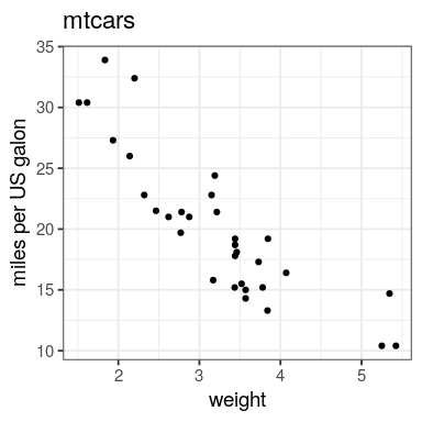
cor(mtcars$mpg, mtcars$wt)

[1] -0.8676594

cor(mtcars$mpg, mtcars$wt, method = "spearman")

[1] -0.886422

cor(mtcars$mpg, mtcars$wt, method = "kendall")

[1] -0.7278321

the Spearman’s rank is valid for samples with n between 7 and 30
for $n>30$ uses the Kendall method

Normality of residuals

assumptions

residuals are independent with similar variance
residuals are normally distributed (hypothesis testing)
diagnostic plot is residuals ~ predicted response
- a: perfect
- b: variance corr with mean, look for log-transform
- c: linear but missing covariate variables
- d: non-linear

plot

source: Logan M.

Diagnostic plots

R base

par(mfrow = (c(2, 2)))
plot(lm(mpg ~ wt, data = mtcars))

Diagnostic plots

ggplot2

library(ggfortify)
autoplot(lm(mpg ~ wt,
            data = mtcars))

Prediction

1/3

ggplot(mtcars, aes(x = wt, y = mpg)) +
  geom_point() +
  geom_smooth(method = "lm", se = FALSE)

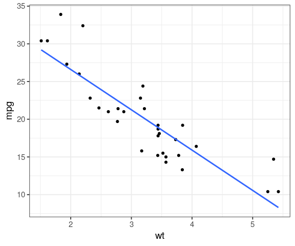
what about a car that weight 4,500 lb (~ 2 tons) ?

Prediction

2/3

fit <- lm(mpg ~ wt, data = mtcars) # create linear model

Use the function coef to extract parameters slope and intercept

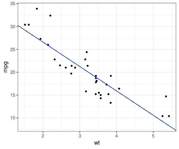
ggplot(mtcars, aes(x = wt, y = mpg)) +
  geom_point() +
  geom_smooth(method = "lm",
              se = FALSE) +
  # new unknown car
  geom_vline(xintercept = 4.5) +  
  geom_hline(yintercept = 
               coef(fit)[1] + coef(fit)[2] * 4.5,
             linetype = "dashed")

Prediction

3/3

predicted fuel consumption

for a specific car weight

coef(fit)[1] + coef(fit)[2] * 4.5

(Intercept) 
     13.235

using the predict function

works with a data frame

predict(fit, data.frame(wt = c(3, 4.5)))

       1        2 
21.25171 13.23500

regression line by hand

`geom_abline()`

line with 2 parameters: abline

ggplot(mtcars, aes(x = wt, y = mpg)) +
  geom_point() +
  geom_abline(slope = coef(fit)[2], intercept = coef(fit)[1]) +
  geom_smooth(method = "lm", se = FALSE, linetype = "dashed")

residuals via broom

`augment`

`broom` functions

tidy(fit), coefficient estimates and hypotheses testing
glance(fit), summary of the model

`augment`

returns the original data + fitted and residuals.

head(augment(fit), 20)

# A tibble: 20 x 10
   .rownames   mpg    wt .fitted .se.fit  .resid   .hat .sigma .cooksd
   <chr>     <dbl> <dbl>   <dbl>   <dbl>   <dbl>  <dbl>  <dbl>   <dbl>
 1 Mazda RX4  21    2.62   23.3    0.634 -2.28   0.0433   3.07 1.33e-2
 2 Mazda RX…  21    2.88   21.9    0.571 -0.920  0.0352   3.09 1.72e-3
 3 Datsun 7…  22.8  2.32   24.9    0.736 -2.09   0.0584   3.07 1.54e-2
 4 Hornet 4…  21.4  3.22   20.1    0.538  1.30   0.0313   3.09 3.02e-3
 5 Hornet S…  18.7  3.44   18.9    0.553 -0.200  0.0329   3.10 7.60e-5
 6 Valiant    18.1  3.46   18.8    0.555 -0.693  0.0332   3.10 9.21e-4
 7 Duster 3…  14.3  3.57   18.2    0.573 -3.91   0.0354   3.01 3.13e-2
 8 Merc 240D  24.4  3.19   20.2    0.539  4.16   0.0313   3.00 3.11e-2
 9 Merc 230   22.8  3.15   20.5    0.540  2.35   0.0314   3.07 9.96e-3
10 Merc 280   19.2  3.44   18.9    0.553  0.300  0.0329   3.10 1.71e-4
11 Merc 280C  17.8  3.44   18.9    0.553 -1.10   0.0329   3.09 2.30e-3
12 Merc 450…  16.4  4.07   15.5    0.719  0.867  0.0558   3.09 2.53e-3
13 Merc 450…  17.3  3.73   17.4    0.610 -0.0502 0.0401   3.10 5.92e-6
14 Merc 450…  15.2  3.78   17.1    0.624 -1.88   0.0419   3.08 8.73e-3
15 Cadillac…  10.4  5.25    9.23   1.26   1.17   0.170    3.09 1.84e-2
16 Lincoln …  10.4  5.42    8.30   1.35   2.10   0.195    3.07 7.19e-2
17 Chrysler…  14.7  5.34    8.72   1.31   5.98   0.184    2.84 5.32e-1
18 Fiat 128   32.4  2.2    25.5    0.783  6.87   0.0661   2.80 1.93e-1
19 Honda Ci…  30.4  1.62   28.7    1.05   1.75   0.118    3.08 2.49e-2
20 Toyota C…  33.9  1.84   27.5    0.942  6.42   0.0956   2.83 2.60e-1
# … with 1 more variable: .std.resid <dbl>

Exercises

Compute

# create linear model
fit <- lm(mpg ~ wt, data = mtcars)
# try this command:
predict(fit)[1:10]

questions

What is it?
compute the residuals
check the sum of square residuals
check normality / homoscedasticity of residuals
plot predicted and residuals with data points and regression line
- original points in black
- predicted points in red
- regression line in blue
- residuals as dashed black segments

residuals

predict call the predicted fuel consumption for the original car weights that were used to built the model.
the difference between original and fitted data are called residuals

`using predict without arguments`

predict(fit)

          Mazda RX4       Mazda RX4 Wag          Datsun 710 
          23.282611           21.919770           24.885952 
     Hornet 4 Drive   Hornet Sportabout             Valiant 
          20.102650           18.900144           18.793255 
         Duster 360           Merc 240D            Merc 230 
          18.205363           20.236262           20.450041 
           Merc 280           Merc 280C          Merc 450SE 
          18.900144           18.900144           15.533127 
         Merc 450SL         Merc 450SLC  Cadillac Fleetwood 
          17.350247           17.083024            9.226650 
Lincoln Continental   Chrysler Imperial            Fiat 128 
           8.296712            8.718926           25.527289 
        Honda Civic      Toyota Corolla       Toyota Corona 
          28.653805           27.478021           24.111004 
   Dodge Challenger         AMC Javelin          Camaro Z28 
          18.472586           18.926866           16.762355 
   Pontiac Firebird           Fiat X1-9       Porsche 914-2 
          16.735633           26.943574           25.847957 
       Lotus Europa      Ford Pantera L        Ferrari Dino 
          29.198941           20.343151           22.480940 
      Maserati Bora          Volvo 142E 
          18.205363           22.427495

Compute predicted and residuals

apply formula

\[residuals = original - predicted\]

my_residuals <- mtcars$mpg - predict(fit)
head(my_residuals)

        Mazda RX4     Mazda RX4 Wag        Datsun 710    Hornet 4 Drive 
       -2.2826106        -0.9197704        -2.0859521         1.2973499 
Hornet Sportabout           Valiant 
       -0.2001440        -0.6932545

`R` has a `residuals` function

that does the job

head(residuals(fit))

        Mazda RX4     Mazda RX4 Wag        Datsun 710    Hornet 4 Drive 
       -2.2826106        -0.9197704        -2.0859521         1.2973499 
Hornet Sportabout           Valiant 
       -0.2001440        -0.6932545

See also summary(residuals(fit)) that shows the upper part of summary(fit)

Residuals: sum of squares

apply formula

\[RSS = \sum_{i=1}^n{(y_i - \hat{y_i})^2}\]

sum(residuals(fit)^2)

[1] 278.3219

to be compared to:

library(broom)
glance(fit)

# A tibble: 1 x 11
  r.squared adj.r.squared sigma statistic  p.value    df logLik   AIC   BIC
      <dbl>         <dbl> <dbl>     <dbl>    <dbl> <int>  <dbl> <dbl> <dbl>
1     0.753         0.745  3.05      91.4 1.29e-10     2  -80.0  166.  170.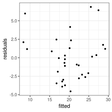
# … with 2 more variables: deviance <dbl>, df.residual <int>

Assessing residuals

diagnostic plots

do you see a pattern?

tibble(fitted = predict(fit),
       residuals = residuals(fit)) %>%
  ggplot() +
  geom_point(aes(fitted, residuals))

what about normality?

tibble(x = residuals(fit)) %>%
  ggplot() +
  stat_qq(aes(sample = x))

Exercise

plot residuals using broom::augment

Goal

We want the predicted values in red, residuals in dashed black

Limits of linear regression

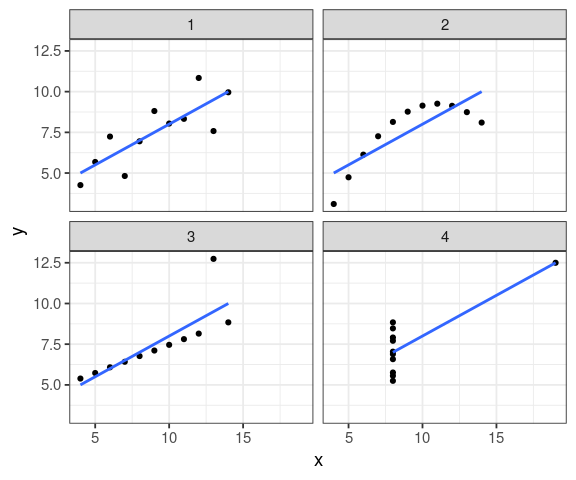
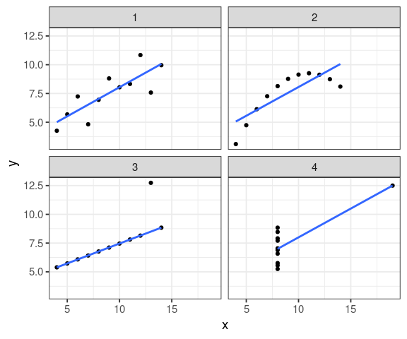
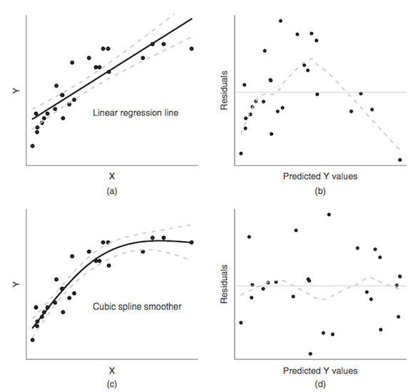
Minimizing the error sum of squares does not resolve everything.

Anscombe demonstrated it by those 4 sets of fake data

anscombe

   x1 x2 x3 x4    y1   y2    y3    y4
1  10 10 10  8  8.04 9.14  7.46  6.58
2   8  8  8  8  6.95 8.14  6.77  5.76
3  13 13 13  8  7.58 8.74 12.74  7.71
4   9  9  9  8  8.81 8.77  7.11  8.84
5  11 11 11  8  8.33 9.26  7.81  8.47
6  14 14 14  8  9.96 8.10  8.84  7.04
7   6  6  6  8  7.24 6.13  6.08  5.25
8   4  4  4 19  4.26 3.10  5.39 12.50
9  12 12 12  8 10.84 9.13  8.15  5.56
10  7  7  7  8  4.82 7.26  6.42  7.91
11  5  5  5  8  5.68 4.74  5.73  6.89

Is this data.frame tidy?

Tidying up Anscombe’s dataset

gather and separate the 4 datasets

anscombe_tidy <- anscombe %>% 
  pivot_longer(
    everything(),
    # .value is a placeholder that 
    # will received x and y
    names_to = c(".value", "set"),
    # regular expression to capture
    names_pattern = "(.)(.)"
  ) %>% 
  as_tibble()
anscombe_tidy

# A tibble: 44 x 3
   set       x     y
   <chr> <dbl> <dbl>
 1 1        10  8.04
 2 2        10  9.14
 3 3        10  7.46
 4 4         8  6.58
 5 1         8  6.95
 6 2         8  8.14
 7 3         8  6.77
 8 4         8  5.76
 9 1        13  7.58
10 2        13  8.74
# … with 34 more rows

reference: David Robinson

Anscombe

regression

perform linear model per group
and broom::tidy to get a tibble back

anscombe_tidy %>%
  group_nest(set) %>%
  mutate(model = map(data, ~ lm(y ~ x, data = .x)),
         tidy = map(model, tidy)) %>%
  unnest(tidy, .drop = TRUE)

Warning: The `.drop` argument of `unnest()` is deprecated as of tidyr 1.0.0.
All list-columns are now preserved.
This warning is displayed once per session.
Call `lifecycle::last_warnings()` to see where this warning was generated.

# A tibble: 8 x 8
  set   data           model term      estimate std.error statistic p.value
  <chr> <list>         <lis> <chr>        <dbl>     <dbl>     <dbl>   <dbl>
1 1     <tibble [11 ×… <lm>  (Interce…    3.00      1.12       2.67 0.0257 
2 1     <tibble [11 ×… <lm>  x            0.500     0.118      4.24 0.00217
3 2     <tibble [11 ×… <lm>  (Interce…    3.00      1.13       2.67 0.0258 
4 2     <tibble [11 ×… <lm>  x            0.5       0.118      4.24 0.00218
5 3     <tibble [11 ×… <lm>  (Interce…    3.00      1.12       2.67 0.0256 
6 3     <tibble [11 ×… <lm>  x            0.500     0.118      4.24 0.00218
7 4     <tibble [11 ×… <lm>  (Interce…    3.00      1.12       2.67 0.0256 
8 4     <tibble [11 ×… <lm>  x            0.500     0.118      4.24 0.00216

compare the $R^2$ using glance

Anscombe

rsquare

anscombe_tidy %>%
  group_nest(set) %>%
  mutate(model = map(data, ~ lm(y ~ x, data = .x)),
         glance = map(model, glance)) %>%
  unnest(glance, .drop = TRUE)

# A tibble: 4 x 14
  set   data  model r.squared adj.r.squared sigma statistic p.value    df
  <chr> <lis> <lis>     <dbl>         <dbl> <dbl>     <dbl>   <dbl> <int>
1 1     <tib… <lm>      0.667         0.629  1.24      18.0 0.00217     2
2 2     <tib… <lm>      0.666         0.629  1.24      18.0 0.00218     2
3 3     <tib… <lm>      0.666         0.629  1.24      18.0 0.00218     2
4 4     <tib… <lm>      0.667         0.630  1.24      18.0 0.00216     2
# … with 5 more variables: logLik <dbl>, AIC <dbl>, BIC <dbl>,
#   deviance <dbl>, df.residual <int>

all $R^2$ are identical!

Anscombe, all models look identical, are they true equally?

ggplot(anscombe_tidy, aes(x, y)) + 
  geom_point() +
  facet_wrap(~ set, ncol = 2) + 
  geom_smooth(method = "lm", se = FALSE)

spurious regressions!

I is correct
II is non-linear
III has one outlier
IV has no trend.

The ADF method

Luc Buissière has a nice way of saying it, from his former teacher Prof. Glenn Morris Univ. of Toronto:

Any Damn Fool should see the effect

If you don’t see a trend, no reason to interpret fake coefficients

r-square, is it useless?

critics from Cosma Shalizi

r-square does not measure goodness of fit

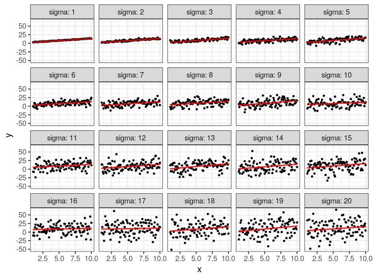
set.seed(123)
x <- seq(1, 10, length.out = 100) # our predictor
# our response; a function of x plus some random noise
map_dfr(seq(0.5, 20, length.out = 20),
        ~ lm(2 + 1.2 * x + rnorm(100, 0, sd = .x) ~ x) %>%
          broom::glance()) %>%
  mutate(sigma = seq(0.5, 20, length.out = 20)) %>%
  ggplot(aes(x = sigma, y = r.squared)) +
  geom_point(size = 2) +
  geom_line()

Clay Ford, University of Viriginia

plotting datasets with increasing sigma

Robust linear models

solve dataset III

`rlm` (M-estimator Huber) weigths the outliers

residuals for data with huge leverage are not squared.
implemented in the library MASS

library(MASS)
anscombe_tidy %>%
  group_nest(set) %>%
  mutate(model = map(data, 
                     ~ rlm(y ~ x, 
                           data = .x)),
         tidy = map(model, tidy)) %>%
  unnest(tidy)

# A tibble: 8 x 7
  set   data              model  term        estimate std.error statistic
  <chr> <list>            <list> <chr>          <dbl>     <dbl>     <dbl>
1 1     <tibble [11 × 2]> <rlm>  (Intercept)    2.98   1.45          2.06
2 1     <tibble [11 × 2]> <rlm>  x              0.506  0.152         3.34
3 2     <tibble [11 × 2]> <rlm>  (Intercept)    3.06   1.31          2.33
4 2     <tibble [11 × 2]> <rlm>  x              0.5    0.137         3.64
5 3     <tibble [11 × 2]> <rlm>  (Intercept)    4.00   0.00404     990.  
6 3     <tibble [11 × 2]> <rlm>  x              0.346  0.000424    816.  
7 4     <tibble [11 × 2]> <rlm>  (Intercept)    3.00   1.26          2.38
8 4     <tibble [11 × 2]> <rlm>  x              0.500  0.132         3.80

rlm plot

ggplot(anscombe_tidy, aes(x, y)) + 
  geom_point() +
  facet_wrap(~ set, ncol = 2) + 
  geom_smooth(method = "rlm", se = FALSE)

assessing coefficients

bootstraps

using tidyeval

boot_set <- function(tib, dataset, rep = 1000) {
  # per set using tidyeval
  filter(tib, set == {{dataset}}) %>%
    # generate 1000 dataset randomly
  modelr::bootstrap(rep) %>%
  mutate(model = map(strap,  ~ lm(y ~ x, .x)),
         tidy  = map(model, tidy)) %>%
  unnest(tidy)
}
#boot_set(anscombe_tidy, "I", 6)
my_sets <- set_names(1:4, nm = c("I", "II", "III", "IV"))
lm_boot <- map_dfr(my_sets, ~ boot_set(anscombe_tidy, .x), .id = "set")

example of bootstrapping

dataset III

transparency

filter(anscombe_tidy, set == 3) %>%
  modelr::bootstrap(12) %>%
  mutate(boot = map(strap, as_tibble)) %>%
  unnest(boot) %>%
  ggplot(aes(x = x, y = y)) +
  geom_point(alpha = 0.6, size = 1.2) +
  geom_smooth(method = "lm", se = FALSE) +
  facet_wrap(~ .id)

plotting coefficient distributions

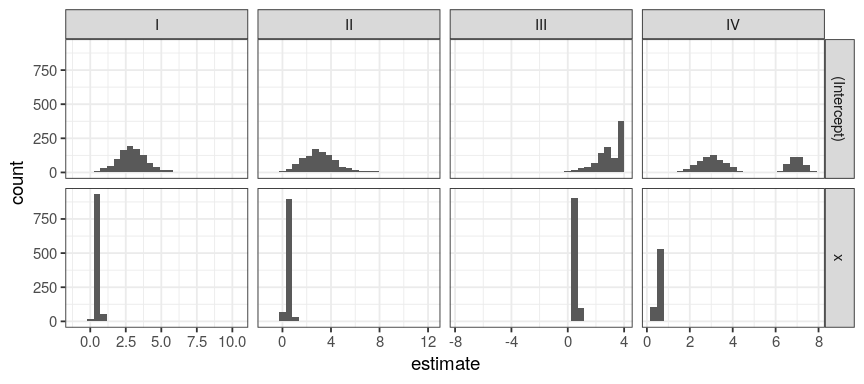
only I is displaying a normal distribution of its coefficients

bootstrap animation

David Robinson

ref: David Robinson@PLOTCON2016

assessing coefficients

cross validation

test partition is either 25 or 50%

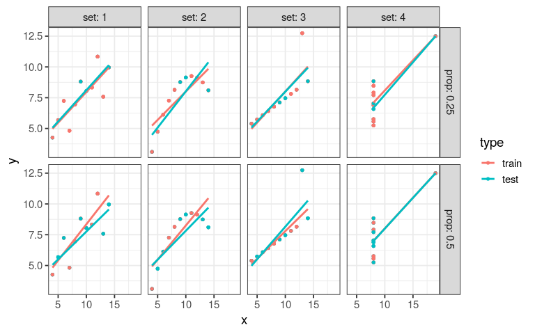
crossing(set = 1:4,
         prop   = c(0.25, 0.5)) %>%
  mutate(cross = map2(set, prop, 
                      ~ crossv_mset(tib = anscombe_tidy, 
                                    dataset = .x, 
                                    prop = .y)),
         MSE_slope = map_dbl(cross, "MSE"),
         MSE_inter = map_dbl(cross, "MSEIntercept")) %>%
  pivot_longer(cols = starts_with("MSE"),
               names_to = "term", 
               values_to = "MSE") %>%
  ggplot(aes(x = set, y = MSE)) +
  geom_col(aes(fill = factor(prop)), 
           position = "dodge") +
  facet_wrap(~ term, ncol = 1) +
  theme(legend.position = "bottom") +
  labs(x = NULL, fill = "prop of test/train",
       title = "Anscombe",
       subtitle = "100 samples per data split")

ref: David Robinson

cross-validation

example of 4 samples

Moving beyond linearity

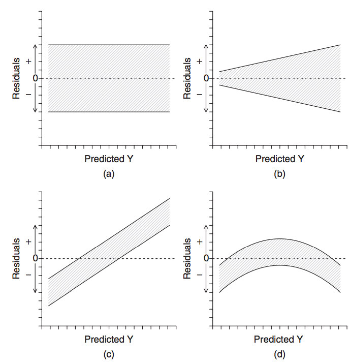
when trend is obviously non-linear, as seen in the residuals

source: Logan M.

Acknowledgements

David Robinson
Luc Buissière

Some of the figures in this presentation are taken from:

An Introduction to Statistical Learning, with applications in R (Springer, 2013) with permission from the authors: G. James, D. Witten, T. Hastie and R. Tibshirani
Biostatistic Design and Analysis Using R. (Wiley-Blackwell, 2011) Murray Logan

Learning objectives

You will learn:

Reading

Regression / Classification

Regression

Classification

Regression

assumptions

global form of modelling

\(f\) and residuals

simulated data ( in blue) and 30 observations

Income could be predicted by years of educations

Residuals

\(f\) is usually never known, use hats (^) for approximations

Prediction

when \(\hat{f}\) is a black box, precision of \(\hat{Y}\) matters

Inference

when estimating \(\hat{f}\) as accurately as possible matters

How to estimate \(f\)?

training / test sets

How to estimate f?

parametric / non-parametric

parametric

non-parametric

Pushing too far non-parametric regressions

risk of overfitting

Linear model, parametric

f is linear

irreducible error, \(\epsilon\)

the usual method is the ordinary least squares

Minimized Residual Sum of Squares

RSS

In the regression \(sales = \beta_0 + \beta_1 \times TV\)

Sum of squares

from lecture 8

demonstrated as a dynamic linear regression

Second step: coefficients estimations

empirical

graphically

advertising dataset

solution

Second step: coefficients estimations

R

Standard Errors of coefficients

RSE

RSE

SE

Standard Errors of coefficients: confidence intervals

meaning, in average

Confidence intervals could be used for hypotheses testing

are they encompassing zero?:

formally, hypotheses (for slope) are:

Assessing the fit

R square

RSE

\(r^2\)

for a simple linear regression,

Correlation versus regression

hypothesis testing

in R default the Pearson \(\rho\) coef

Normality of residuals

assumptions

plot

Diagnostic plots

R base

Diagnostic plots

ggplot2

Prediction

1/3

Prediction

2/3

Prediction

3/3

predicted fuel consumption

using the predict function

regression line by hand

geom_abline()

line with 2 parameters: abline

residuals via broom

augment

`geom_abline()`

`augment`

`broom` functions

`augment`

`using predict without arguments`

`R` has a `residuals` function

`rlm` (M-estimator Huber) weigths the outliers