Biostatistic - introduction

October 2019

Biostatistics

You will learn to:

basics of statistic
term definition
theoritical distributions
compare 2 samples

Reading

Book

Statistics. An introduction using R by Michael J. Crawley

An Introduction to Statistical Learning by James, Witten, Hastie & Tibshirani

Biostatistic Design and Analysis Using R by Murray Logan

Statistic

Clearly identify response variables from explanatory (or predictor) variables.

below, which is explanatory/response?

blood pressure
cholesterol blood concentration

solution

blood pressure, response, y axis
cholesterol blood concentration, explanatory x axis

Fuel consumption and car weight example

`geom_smooth()` with linear modelling

ggplot(mtcars, aes(x = wt, y = mpg)) +
  geom_point() +
  geom_smooth(method = "lm")

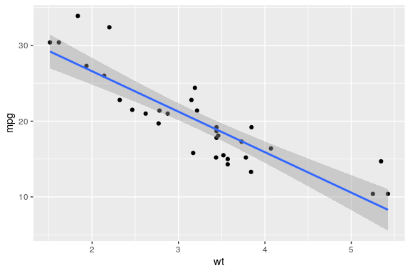
Miles per US galon (mpg) is the response
Weigth (wt) is a predictor

Correlation

variable order does not matter

cor.test(mtcars$mpg, mtcars$wt)

    Pearson's product-moment correlation

data:  mtcars$mpg and mtcars$wt
t = -9.559, df = 30, p-value = 1.294e-10
alternative hypothesis: true correlation is not equal to 0
95 percent confidence interval:
 -0.9338264 -0.7440872
sample estimates:
       cor 
-0.8676594

cor.test(mtcars$wt, mtcars$mpg)

    Pearson's product-moment correlation

data:  mtcars$wt and mtcars$mpg
t = -9.559, df = 30, p-value = 1.294e-10
alternative hypothesis: true correlation is not equal to 0
95 percent confidence interval:
 -0.9338264 -0.7440872
sample estimates:
       cor 
-0.8676594

Derive an equation to predict response y

linear regression

summary(lm(mtcars$mpg ~ mtcars$wt))

Call:
lm(formula = mtcars$mpg ~ mtcars$wt)

Residuals:
    Min      1Q  Median      3Q     Max 
-4.5432 -2.3647 -0.1252  1.4096  6.8727 

Coefficients:
            Estimate Std. Error t value Pr(>|t|)    
(Intercept)  37.2851     1.8776  19.858  < 2e-16 ***
mtcars$wt    -5.3445     0.5591  -9.559 1.29e-10 ***
---
Signif. codes:  0 '***' 0.001 '**' 0.01 '*' 0.05 '.' 0.1 ' ' 1

Residual standard error: 3.046 on 30 degrees of freedom
Multiple R-squared:  0.7528,    Adjusted R-squared:  0.7446 
F-statistic: 91.38 on 1 and 30 DF,  p-value: 1.294e-10

\(cor^2\) = \(r^2\)

cor(mtcars$wt, mtcars$mpg)

[1] -0.8676594

cor(mtcars$wt, mtcars$mpg)^2

[1] 0.7528328

Correlation is not causality

source: spurious correlations

Today’s Logic Lesson : Correlation v. Causation pic.twitter.com/ZJaLACw8tB
— Philosophy Matters (@PhilosophyMttrs) 30 septembre 2018

Variables

Continuous

any real numbered value

women$height[1:10]

 [1] 58 59 60 61 62 63 64 65 66 67

Categorical

factor with levels

ToothGrowth$supp[1:10]

 [1] VC VC VC VC VC VC VC VC VC VC
Levels: OJ VC

str(ToothGrowth$supp[1:10])

 Factor w/ 2 levels "OJ","VC": 2 2 2 2 2 2 2 2 2 2

Convert numbers to categories

mtcars$cyl[1:10]

 [1] 6 6 4 6 8 6 8 4 4 6

factor(mtcars$cyl[1:10])

 [1] 6 6 4 6 8 6 8 4 4 6
Levels: 4 6 8

Convert factor to strings

as.character(ToothGrowth$supp[1:10])

 [1] "VC" "VC" "VC" "VC" "VC" "VC" "VC" "VC" "VC" "VC"

Appropriate statistical methods

Explanatory	Response	Method
continuous	continuous	regression
continuous	continuous	correlation
categorical	continuous	analysis of variance (anova)
continuous / categorical	continuous	analysis of covariance (ancova)
continuous	proportion	logistic regression
continuous	count	logit regression
continuous	time-at-death	survival analysis

What for?

hypotheses

A good hypothesis is a falsifiable hypothesis Karl Popper

Which of these two is a good hypothesis?

#1

There are vultures in the local park

#2

There are no vultures in the local park

Null hypotheses

the null hypothesis, \(H_0\), is similar to “nothing is happening”

What matters: null hypothesis must be falsifiable.
We reject the null hypothesis when the data shows it is sufficiently unlikely.

examples

comparison of two means
correlation between x and y
comparison of three means
comparison of two proportions
slopes are not zero

Significance

characteristics

sufficiently unlikeliness is determined by the significance of statistical tests
if the alternate hypothesis \(H_1\) occurs more than 5% of the time, we reject \(H_0\)
significance is a threshold chosen by the user
has to be compared to the p value obtained

p values are probabilities (\(0 \leq p \leq 1\)) that a particular result occurred by chance if \(H_0\) is true.

if \(H_0\) is true is almost never true. Instead a mixture of null and alternative hypotheses

p > 0.05 tells you the experiment is strictly underpowered and shouldn't be interpreted at all.

p < 0.001 tells you that you've found something worth running multiple studies on.
— John Myles White (@johnmyleswhite) 26 janvier 2018

Type of errors and interpretation

Two types of errors can be made

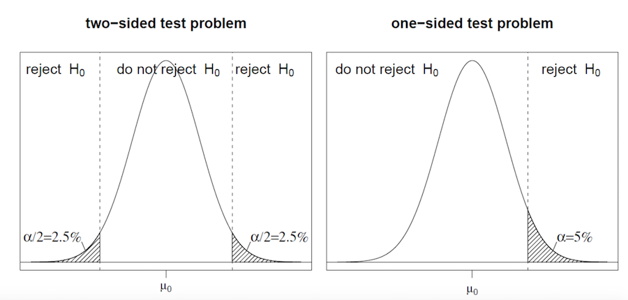
and are made at a certain threshold

reject \(H_0\) while it was true, type I
accept \(H_0\) while it was false, type II

Errors types

Attaching package: 'kableExtra'

The following object is masked from 'package:dplyr':

    group_rows

Warning: funs() is soft deprecated as of dplyr 0.8.0
Please use a list of either functions or lambdas: 

  # Simple named list: 
  list(mean = mean, median = median)

  # Auto named with `tibble::lst()`: 
  tibble::lst(mean, median)

  # Using lambdas
  list(~ mean(., trim = .2), ~ median(., na.rm = TRUE))
This warning is displayed once per session.

	Null hypothesis is
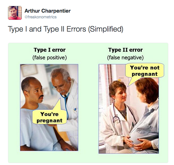
decision on H0	True	False
Reject	Type I error	Correct
Accept	Correct	Type II error

Which one is

the false positive?
the false negative?

the power of a test is \(1 - \beta\)

Power of t-tests

1/10 difference needs 100 more n

Intial tweet by John Myles White, R code modified from the gist by David Robinson.

Assessing the true difference of means

fixed standard deviation = 1

crossing(n = 3:30,
         delta = NULL,
         sig.level = .05,
         power = seq(.3, .9, .2),
         sd = 1,
         type = c("two.sample")) %>%
  pmap(.l = ., .f = power.t.test) %>%
  map_df(tidy) %>%
  ggplot(aes(x = n, y = delta)) +
  geom_line(aes(colour = percent(power)),
            size = 1.1) +
  geom_hline(yintercept = 2^0.5, 
             linetype = "dashed") +
  annotate("text", x = 25, y = 1.6, 
   label = "log[2]*\" = 0.5\"",
   parse = TRUE, size = 6) +
  scale_y_continuous(labels = percent) +
  scale_x_continuous(breaks = c(3,5,10,20,30)) +
  theme_minimal(20) +
  labs(x = "# observations (both samples)",
       y = "true difference of means",
       color = "power",
       title = "Power of 2-samples t-test ",
       subtitle = "for sd = 1")

Generate data

sample of population

Your experimental design should take care of two key concepts

replication

to increase reliability
capture as many events as you can afford
must be independent

randomization

to reduce bias, cannot test everything

others

appropriate controls
modelling:
- parsimony
- as few parameters as possible
- linear over non-linear

Mind pseudo-replication

source asbmb.org

Population versus samples

terms

parameter

characteristic of a population
greek letters
mean \(\mu\), sd \(\sigma\), var \(\sigma^2\)

statistic

characteristic of a sample
latin letters
mean \(\bar{x}\), sd \(s\), var \(s^2\)

cliffnotes

models

simulate population

this implies that we have models, distributions that we know and can be used to assess our data.

normal distribution

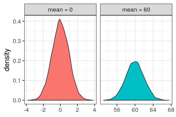
Two parameters

mean
standard deviation
simulation

Student t distribution

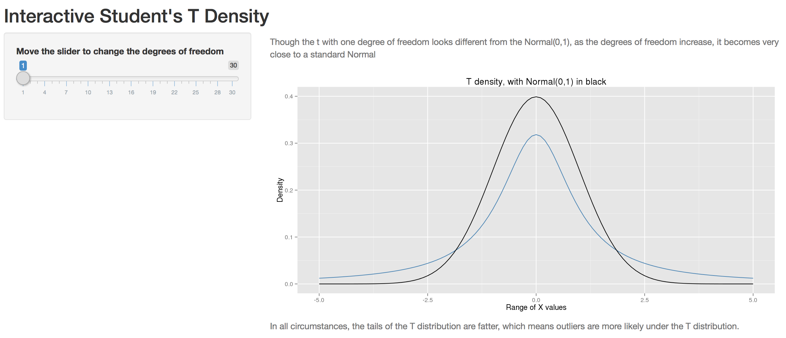
For smaller sample sizes, one more parameter: degrees of freedom. \[df = n - p\]

\(n\) is the sample size
\(p\) nb parameters estimated from data

Thus, 3 parameters:

df
mean
standard deviation

Normal versus t distribution

Larger incertainty leads to bigger tails

comparison normal versus student

simulation

Degrees of freedom

Let’s say we have 5 observations with a known average of 4.

first, fetch a 2

1	2	3	4	5
2

average = 2

second, fetch a 7

1	2	3	4	5
2	7

average = 4.5

third, fetch a 4

1	2	3	4	5
2	7	4

average = 4.3333333

fourth, fetch a 0

1	2	3	4	5
2	7	4	0

average = 3.25

Degrees of freedom

But, now only one available spot

and the average must be 4

for 5 elements

we must have a sum of 20.

\[20 - (2 + 7 + 4 + 0) = 7\]

final

1	2	3	4	5
2	7	4	0	7

average = 4

formula

\[df = n - 1 = 5 - 1 = 4\]

Mean / Median / Mode

summary statistics

mean

suffers from extreme values

\[\mu = \frac{\sum x}{n}\]

median

middle value, sort values:

even length: average of the two centered values
odd length: middle value

mode

value that occurs the most frequently

Mean / Median

plotted

set.seed(123)
dens <- data_frame(x = c(rnorm(500), rnorm(200, 3, 3)))

Warning: `data_frame()` is deprecated, use `tibble()`.
This warning is displayed once per session.

ggplot(dens) +
  geom_line(aes(x), stat = "density") +
  geom_vline(aes(xintercept = mean(x), colour = "mean"), size = 1.1) +
  geom_vline(aes(xintercept = median(x), colour = "median"), size = 1.1) -> p
p

with mode

dens_mode <- density(dens$x)$x[which.max(density(dens$x)$y)]
p + geom_vline(aes(xintercept = dens_mode, colour = "mode"), size = 1.1)

Variance

measures variability

dispersion around a central tendency.
measured as the sum of differences to the mean, use squares to get rid of sign issue.

formula

\[variance = \frac{sum\,of\,squares}{degrees\,of\,freedom}\]

dispersion are also called residuals

\[residual = observed\,value - predicted\,value\]

Sum of squares

demonstrated as a dynamic linear regression

Standard error of the mean

unreliability of measures are called standard errors

For the mean, standard errors decrease when the sample size increases
could be written as:

x has a mean of \[3.0 \pm 0.365 (1 s.e, n = 10)\]

formula

\[SE_\bar{y} = \sqrt{\frac{s^2}{n}}\]

Confidence intervals

unreliability could be represented as confidence intervals

Intervals go wider when the unreliability goes up.
confidence intervals are always two-tailed
usually associated to the t values from the Student’s distribution

A CI is how many t standard error to be expected for a given interval

formula

\[confidence\,interval = t \times standard\,error\]

Confidence interval

garden example from J. Crawley

garden

# A tibble: 10 x 3
   gardenA gardenB gardenC
     <dbl>   <dbl>   <dbl>
 1       3       5       3
 2       4       5       3
 3       4       6       2
 4       3       7       1
 5       2       4      10
 6       3       4       4
 7       1       3       3
 8       3       5      11
 9       5       6       3
10       2       5      10

mean for garden A

mean(garden$gardenA)

[1] 3

t 2.5% for \(\;\alpha = 0.05\)

qt(0.025, df = 9)

[1] -2.262157

qt(0.975, df = 9)

[1] 2.262157

qt(0.975, df = 9) * sqrt(var(garden$gardenA) / length(garden$gardenA))

[1] 0.826023

confidence interval, mean gardenA

\(\;\bar{x} = 3.0 \pm 0.83 (CI_{95\%})\)

Parameters / Statistics

population

mean, \(\mu = \frac{\sum(x)}{N}\)
variance, \(\sigma^2 = \frac{\sum(x - \mu)^2}{N}\)
standard deviation, \(\sigma = \sqrt{\frac{\sum(x - \mu)^2}{N}}\)

sample (p = 1, mean estimated)

mean, \(\bar{x} = \frac{\sum(x)}{n}\)
variance, \(s^2 = \frac{\sum(x - \bar{x})^2}{n - 1}\)
standard deviation, \(s = \sqrt{\frac{\sum(x - \bar{x})^2}{n - 1}}\)

Functions in R

base

mean()
var()
sd()
# median absolute deviation
mad()

example

a <- garden$gardenA
mean(a)

[1] 3

var(a)

[1] 1.333333

sd(a)

[1] 1.154701

mad(a) # median absolute deviation

[1] 1.4826

Central Limit Theorem

with more replicates -> converge to the average and to a normal distribution

https://rpubs.com/nishantsbi/112044 by nishantsbi

Normal distribution

properties

median = mean = mode
\(1 \sigma = 68\%\)
\(2 \sigma = 95\%\)
\(3 \sigma = 99\%\)

z-scores

also called standardized scores, they refer to how many standard deviation to the mean.

Formula to obtain a z-score from a normal distribution

\[z = \frac{x - \mu}{\sigma}\]

z-scores

using R

with 2 \(\sigma\)

1 - 2 * pnorm(-2)

[1] 0.9544997

more precisely

z <- qnorm(0.025)
z

[1] -1.959964

1 - 2 * pnorm(z)

[1] 0.95

relationship between `p, q, r` for the normal distribution

by Eric Koncina

Working example

Suppose we have measured the height of 100 people: The mean height is 170 cm and the standard deviation is 8 cm.

how much of the population is shorter than 160 cm?

Solution

Calculate the z-score from the distribution

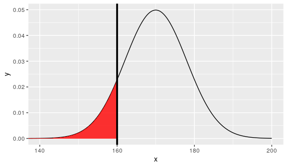
z <- (160 - 170) / 8
z

[1] -1.25

z is a negative value

what can we predict about the proportion of people?
More or less of 50%?

from z to p, associated probability

i.e area under the bell shape.

pnorm(z)

[1] 0.1056498

paste(round(pnorm(z) * 100, 2), "%")

[1] "10.56 %"

One / Two side tests

One sample

assumption: normality of the residuals

set.seed(123)
rn <- rnorm(100)
shapiro.test(rn)

    Shapiro-Wilk normality test

data:  rn
W = 0.99388, p-value = 0.9349

one sample t-test comparison to mean = 0

t.test(garden$gardenA)

    One Sample t-test

data:  garden$gardenA
t = 8.2158, df = 9, p-value = 1.788e-05
alternative hypothesis: true mean is not equal to 0
95 percent confidence interval:
 2.173977 3.826023
sample estimates:
mean of x 
        3

One way t-test

Test if the mean of a one sample if different from a population parameter

\[\mu\ != \bar{x}\]

using R

mean(mtcars$mpg)

[1] 20.09062

t.test(mtcars$mpg, mu = 18, alternative = "two.sided")

    One Sample t-test

data:  mtcars$mpg
t = 1.9622, df = 31, p-value = 0.05876
alternative hypothesis: true mean is not equal to 18
95 percent confidence interval:
 17.91768 22.26357
sample estimates:
mean of x 
 20.09062

compare 2 means

Two samples

comparing variances

assumptions

normality
independence
similar variances

Fisher’s F test

var.test(sample1, sample2)

Divide the larger variance by the smaller one.

compare the variances of garden A & C

using the garden dataset.

Variance test

doing it by hand

var(garden$gardenA)

[1] 1.333333

var(garden$gardenC)

[1] 14.22222

F.ratio <- var(garden$gardenC) / var(garden$gardenA)
F.ratio

[1] 10.66667

F distribution

tibble(x = seq(-2, 10, length.out = 500),
       y = df(x, 9, 9)) %>%
  ggplot() +
  geom_line(aes(x = x, y = y)) +
  theme_bw(18)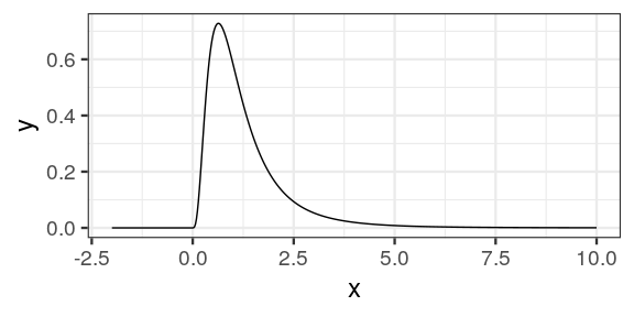

why no values < 0?

no values < 0, mind the degrees of freedom!

Variance test

doing it by hand

Hypothesis

\(H_0\): the two variances are not statistically different
\(H_1\): the two variances are statistically different

define the critical value of F distribution for a risk of \(alpha = 0.05\)

qf(0.975, 9, 9)

[1] 4.025994

Could you already accept or reject \(H_0\)?

Variance test

doing it by hand

compute the exact p-value

2 * (1 - pf(F.ratio, 9, 9))

[1] 0.001624199

now using the build-in R function

var.test(garden$gardenA, garden$gardenC)

    F test to compare two variances

data:  garden$gardenA and garden$gardenC
F = 0.09375, num df = 9, denom df = 9, p-value = 0.001624
alternative hypothesis: true ratio of variances is not equal to 1
95 percent confidence interval:
 0.02328617 0.37743695
sample estimates:
ratio of variances 
           0.09375

Student’s t test

comparing two means

assumptions

the two samples must be independent
the two variances have to be similar
error must be normally distributed

methods

study design
F test
normality test

if not normal?

non parametric tests

Wilcoxon rank sum test
- samples must be independent
- errors are not normally distributed

Student’s t test

rationale

for small sample size (n < 30)
concern most of biological studies
inferences needed from population variance \(\,\sigma^2\) using the sample variance \(\,s^2\).
more uncertainty, since population parameters cannot be known.

The t test statistic

provides the number of standard error by which two sample means are separated.

\[ t = \frac{difference\,between\,two\,means}{standard\,error\,of\,the\,difference} = \frac{ \overline{y_A} - \overline{y_B}}{s.e_{diff}}\]

Standard error of a difference

For two independent samples

the variance of their difference is the sum of their variances.

\[s.e_{diff} = \sqrt{\frac{s_A^2}{n_A} + \frac{s_B^2}{n_B}}\]

Example

garden

GardenA and gardenC have significant different variances

but let’s see for gardenA and B

A vs B

var.test(garden$gardenA, garden$gardenB)

    F test to compare two variances

data:  garden$gardenA and garden$gardenB
F = 1, num df = 9, denom df = 9, p-value = 1
alternative hypothesis: true ratio of variances is not equal to 1
95 percent confidence interval:
 0.2483859 4.0259942
sample estimates:
ratio of variances 
                 1

testing normality

library(broom)
tidy(shapiro.test(garden$gardenA))

# A tibble: 1 x 3
  statistic p.value method                     
      <dbl>   <dbl> <chr>                      
1     0.953   0.703 Shapiro-Wilk normality test

tidy(shapiro.test(garden$gardenB))

# A tibble: 1 x 3
  statistic p.value method                     
      <dbl>   <dbl> <chr>                      
1     0.953   0.703 Shapiro-Wilk normality test

Example

garden

independence

since two different gardens

compute it!

1st diff of means

diff <- mean(garden$gardenA) - mean(garden$gardenB)
diff

[1] -2

compute t statistic

t <- diff / (sqrt((var(garden$gardenA) / 10) + (var(garden$gardenB) / 10)))
t # sign does not matter, how many df?

[1] -3.872983

deduced p-value

2 * pt(t, df = 18)

[1] 0.001114539

Compare 2 means, using R

garden example

Welch correction

unequal variance is compensated by lowering df
is ON by default

t.test(garden$gardenA, garden$gardenB,
       var.equal = FALSE)

    Welch Two Sample t-test

data:  garden$gardenA and garden$gardenB
t = -3.873, df = 18, p-value = 0.001115
alternative hypothesis: true difference in means is not equal to 0
95 percent confidence interval:
 -3.0849115 -0.9150885
sample estimates:
mean of x mean of y 
        3         5

t.test(garden$gardenA, garden$gardenB,
       var.equal = TRUE)

    Two Sample t-test

data:  garden$gardenA and garden$gardenB
t = -3.873, df = 18, p-value = 0.001115
alternative hypothesis: true difference in means is not equal to 0
95 percent confidence interval:
 -3.0849115 -0.9150885
sample estimates:
mean of x mean of y 
        3         5

Two dependent samples

paired t test

the independence assumption is violated when the samples share more than they should.
Such as:
- two samples from a same individual
- two samples from the same biotope …

parametric test

t.test(x, y, paired = TRUE)

= a one-sample t test with the difference of samples

Mann and Whitney rank sum

non-parametric

When?

when the errors are not normally distributed

Non-parametric alternative to the Student’s t test

wilcox.test()

default paired = FALSE, for independent samples, aka Mann-Whitney’s test.
with paired = TRUE, for dependent samples, aka Wilcoxon.
process:
- label the values
- mix
- rank them. The main issue is ties.

Wilcoxon

example

garden %>%
  # go for long format
  gather(garden, ozone) %>% 
  # focus on A and B
  filter(garden != "gardenC") %>% 
  mutate(rank = rank(ozone, ties.method = "average")) %>% 
  # do the grouping AFTER ranking
  group_by(garden) %>%
  # get the sum!
  summarise(sum(rank))

# A tibble: 2 x 2
  garden  `sum(rank)`
  <chr>         <dbl>
1 gardenA          66
2 gardenB         144

compared to the critical value

value has to be < for both \(n = 10\) samples

qwilcox(0.975, 10, 10)

[1] 76

conclusions

compare this critical value to the 2 sum(rank).
if one of sum is higher than 76 -> we reject \(H_0\).
Garden A and B have different means.

Non-parametric versus parametric

if we compare the two p-values we obtain

bind_rows(
  tidy(wilcox.test(
    garden$gardenA,
    garden$gardenB)),
  tidy(t.test(
    garden$gardenA,
    garden$gardenB)))

# A tibble: 2 x 10
  statistic p.value method alternative estimate estimate1 estimate2
      <dbl>   <dbl> <chr>  <chr>          <dbl>     <dbl>     <dbl>
1     11    0.00299 Wilco… two.sided         NA        NA        NA
2     -3.87 0.00111 Welch… two.sided         -2         3         5
# … with 3 more variables: parameter <dbl>, conf.low <dbl>,
#   conf.high <dbl>

non-parametric tests are more conservative with less power

for \(n=3\) power is zero. Minimum is \(n=4\)

Compare two distributions

assumption on distribution shapes, even if unknown

non parametric test
Kolmogorov-Smirnov test
compares 2 distributions by working on their cumulative distribution function

ks.test()

tibble(x = seq(-5, 5, length.out = 100),
       `1` = pnorm(x),
       `2` = pnorm(x, 0, 2),
       `3` = pnorm(x,  0, 3)) %>%
  gather(sd, y, -x) %>%
  ggplot(aes(x, y, colour = sd)) +
  geom_line() +
  theme_bw(18)

Biostatistics

You will learn to:

Reading

Book

Statistic

below, which is explanatory/response?

solution

Fuel consumption and car weight example

geom_smooth() with linear modelling

Correlation

variable order does not matter

Derive an equation to predict response y

linear regression

\(cor^2\) = \(r^2\)

Correlation is not causality

Variables

Continuous

Categorical

Convert numbers to categories

Convert factor to strings

Appropriate statistical methods

What for?

hypotheses

#1

#2

Null hypotheses

the null hypothesis, \(H_0\), is similar to “nothing is happening”

examples

Significance

characteristics

Type of errors and interpretation

Two types of errors can be made

Errors types

Which one is

Power of t-tests

1/10 difference needs 100 more n

Assessing the true difference of means

fixed standard deviation = 1

Generate data

sample of population

replication

randomization

others

Mind pseudo-replication

Population versus samples

terms

parameter

statistic

models

simulate population

normal distribution

Student t distribution

Normal versus t distribution

comparison normal versus student

Degrees of freedom

first, fetch a 2

second, fetch a 7

third, fetch a 4

fourth, fetch a 0

Degrees of freedom

But, now only one available spot

for 5 elements

final

formula

Mean / Median / Mode

summary statistics

mean

median

mode

Mean / Median

plotted

with mode

Variance

measures variability

formula

dispersion are also called residuals

Sum of squares

demonstrated as a dynamic linear regression

Standard error of the mean

unreliability of measures are called standard errors

`geom_smooth()` with linear modelling

relationship between `p, q, r` for the normal distribution