Data transformation

October 2019

Data transformation

Introduction

Preparing data is the most time consuming part of of data analysis

`dplyr` is a tool box for working with data in tibbles/data frames

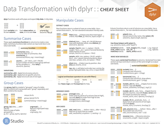
The most import data manipulation operations are covered
- Selection and manipulation
  - Selection and manipulation of
  - observations,
  - variables and
  - values.
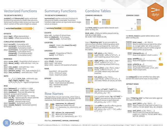
- Summarizing
- Grouping
- Joining and intersecting tibbles
In a workflow typically follows reshaping operations from tidyr
Fast, by writing key pieces in C++ (using Rcpp)
Standard interfaces to database (dbplyr) or data.table (dtplyr).

Preparing data is the most time consuming part of of data analysis!

Essential part of understanding data, hard to avoid.

Learning objectives

You will learn to:

Learn the basic vocabulary of dplyr
Exercise commands
Translating questions into data manipulation statements
A peak at some feature not as frequently used
Revisit the tidyr package

Preparing your environment

The dataset

Genes from chromosome 21
Was downloaded from bioMart, saved as a .csv.
load the provided csv file
assign to the name genes_by_transcripts

read data

genes_by_transcripts <- read_csv("data/genes_by_transcripts.csv")

Parsed with column specification:
cols(
  ensembl_gene_id = col_character(),
  ensembl_transcript_id = col_character(),
  chromosome_name = col_double(),
  start_position = col_double(),
  end_position = col_double(),
  hgnc_symbol = col_character(),
  hgnc_id = col_character(),
  strand = col_double(),
  gene_biotype = col_character()
)

`biomaRt` is part of bioconductor

FYI (not to be run)

for install

# install if missing
# install.packages("BiocManager")
BiocManager::install("biomaRt")

Gene info from chromosome 21 using `biomaRt`

library(biomaRt)
gene_mart <- useMart(biomart = "ENSEMBL_MART_ENSEMBL",
                     host = "www.ensembl.org")
gene_set <- useDataset(gene_mart ,
                       dataset = "hsapiens_gene_ensembl")
# choose desired fields
genes_by_transcripts <- getBM(mart = gene_set,
                  attributes = c("ensembl_gene_id",
                                 "ensembl_transcript_id",
                                 "chromosome_name",
                                 "start_position",
                                 "end_position",
                                 "hgnc_symbol",
                                 "hgnc_id",
                                 "strand",
                                 "gene_biotype"
                  ), # here narrow query to chr21
                  filters = "chromosome_name",
                  values = "21"
)

`dplyr` cheatsheets

http://perso.ens-lyon.fr/lise.vaudor/dplyr/

Reminder: Pipes in R

magrittr

Without pipe

verb(subject, complement)

With pipe

subject %>% verb(complement)

Example adapted from Romain François

Remark

tidyverse functions are consistently designed to work with %>%:

data (subject) is the first argument.

Graphical summary

http://perso.ens-lyon.fr/lise.vaudor/dplyr/

Outline

Reference tibble

Here, we will use the the genes_by_transcripts tibble to show some of the main functions (verbs) provided by dplyr

Use `dplyr()` to:

Inspect your tibble (glimpse())
Select specific columns (select())
Filter out a subset of rows (filter())
Change or add columns (mutate())
Group observations by a grouping variable (group_by())
Get a summary (in particular per group) (summarise())
Join two distinct tibbles by a common column (left_join(), right_join() and full_join())

Inspect tibbles

`glimpse()`

Shows some values and the type of each column.
The Environment tab in RStudio tab does it too (for example, click on the blue button left to your object genes_by_transcripts to expand the view)
Similar to the base::str() function

glimpse(genes_by_transcripts)

Observations: 2,436
Variables: 9
$ ensembl_gene_id       <chr> "ENSG00000251972", "ENSG00000274046", "ENSG0000…
$ ensembl_transcript_id <chr> "ENST00000516163", "ENST00000617336", "ENST0000…
$ chromosome_name       <dbl> 21, 21, 21, 21, 21, 21, 21, 21, 21, 21, 21, 21,…
$ start_position        <dbl> 25943044, 7092616, 13724189, 33550662, 8208473,…
$ end_position          <dbl> 25943145, 7092716, 13724274, 33550728, 8208652,…
$ hgnc_symbol           <chr> "RNU6-123P", NA, "MIR8069-2", "MIR6501", "MIR36…
$ hgnc_id               <chr> "HGNC:47086", NA, "HGNC:50836", "HGNC:50033", "…
$ strand                <dbl> -1, 1, 1, 1, 1, 1, -1, 1, 1, 1, 1, 1, 1, 1, 1, …
$ gene_biotype          <chr> "snRNA", "misc_RNA", "miRNA", "miRNA", "miRNA",…

Selecting columns

`select()`

Select the columns you want: select(tibble, your_column1, ...)

select example

select(genes_by_transcripts, hgnc_symbol, start_position, end_position)

# A tibble: 2,436 x 3
   hgnc_symbol start_position end_position
   <chr>                <dbl>        <dbl>
 1 RNU6-123P         25943044     25943145
 2 <NA>               7092616      7092716
 3 MIR8069-2         13724189     13724274
 4 MIR6501           33550662     33550728
 5 MIR3648-1          8208473      8208652
 6 RNU4-45P          22205192     22205332
 7 <NA>              32841861     32841995
 8 <NA>              28743208     28743291
 9 UBASH3A           42403447     42447681
10 UBASH3A           42403447     42447681
# … with 2,426 more rows

Selecting columns using `select()`

helper functions

contains() (a character sequence)
starts_with() (a character sequence)
ends_with() (a character sequence)
one_of() names in a character vector
matches() (using regular expressions)
everything() all remaining columns

select(genes_by_transcripts, ends_with("position"))

# A tibble: 2,436 x 2
   start_position end_position
            <dbl>        <dbl>
 1       25943044     25943145
 2        7092616      7092716
 3       13724189     13724274
 4       33550662     33550728
 5        8208473      8208652
 6       22205192     22205332
 7       32841861     32841995
 8       28743208     28743291
 9       42403447     42447681
10       42403447     42447681
# … with 2,426 more rows

Tip

You can combine different helpers

select(genes_by_transcripts, contains("gene"), starts_with("hgnc"))

# A tibble: 2,436 x 4
   ensembl_gene_id gene_biotype   hgnc_symbol hgnc_id   
   <chr>           <chr>          <chr>       <chr>     
 1 ENSG00000251972 snRNA          RNU6-123P   HGNC:47086
 2 ENSG00000274046 misc_RNA       <NA>        <NA>      
 3 ENSG00000278618 miRNA          MIR8069-2   HGNC:50836
 4 ENSG00000284448 miRNA          MIR6501     HGNC:50033
 5 ENSG00000275708 miRNA          MIR3648-1   HGNC:38941
 6 ENSG00000202339 snRNA          RNU4-45P    HGNC:46981
 7 ENSG00000207098 snoRNA         <NA>        <NA>      
 8 ENSG00000283300 snRNA          <NA>        <NA>      
 9 ENSG00000160185 protein_coding UBASH3A     HGNC:12462
10 ENSG00000160185 protein_coding UBASH3A     HGNC:12462
# … with 2,426 more rows

Selecting columns using `select()`

Dropping columns (negative selection)

We can drop columns by “negating” their names.
Works also with the helper functions

negative selection example

select(genes_by_transcripts, -strand, -starts_with("ensembl"), -ends_with("id"))

# A tibble: 2,436 x 5
   chromosome_name start_position end_position hgnc_symbol gene_biotype  
             <dbl>          <dbl>        <dbl> <chr>       <chr>         
 1              21       25943044     25943145 RNU6-123P   snRNA         
 2              21        7092616      7092716 <NA>        misc_RNA      
 3              21       13724189     13724274 MIR8069-2   miRNA         
 4              21       33550662     33550728 MIR6501     miRNA         
 5              21        8208473      8208652 MIR3648-1   miRNA         
 6              21       22205192     22205332 RNU4-45P    snRNA         
 7              21       32841861     32841995 <NA>        snoRNA        
 8              21       28743208     28743291 <NA>        snRNA         
 9              21       42403447     42447681 UBASH3A     protein_coding
10              21       42403447     42447681 UBASH3A     protein_coding
# … with 2,426 more rows

Filtering out rows

with repositioning of a column

`filter()`

Take a look at the amyloid precursor protein gene APP
Place the hgnc_symbol column 1st using select() and everything()

filter(genes_by_transcripts, hgnc_symbol == "APP") %>% 
  select(hgnc_symbol, everything())

# A tibble: 17 x 9
  hgnc_symbol ensembl_gene_id ensembl_transcr… chromosome_name start_position
  <chr>       <chr>           <chr>                      <dbl>          <dbl>
1 APP         ENSG00000142192 ENST00000346798               21       25880550
2 APP         ENSG00000142192 ENST00000354192               21       25880550
3 APP         ENSG00000142192 ENST00000348990               21       25880550
# … with 14 more rows, and 4 more variables: end_position <dbl>, hgnc_id <chr>,
#   strand <dbl>, gene_biotype <chr>

Row vs column selection

filter() acts on rows
select() acts on columns

Filtering out rows

multiple conditions, AND (`&`)

multiple conditions: AND

comma separated conditions are equivalent to & (AND)
Filter genes located in a particular range:

filter(genes_by_transcripts, start_position > 1.05e7, end_position < 1.1e7)

# A tibble: 9 x 9
  ensembl_gene_id ensembl_transcr… chromosome_name start_position end_position
  <chr>           <chr>                      <dbl>          <dbl>        <dbl>
1 ENSG00000273872 ENST00000614260               21       10612455     10613379
2 ENSG00000278678 ENST00000616920               21       10576292     10576587
3 ENSG00000277282 ENST00000622028               21       10649400     10649835
4 ENSG00000276556 ENST00000611755               21       10640028     10640338
5 ENSG00000274391 ENST00000622113               21       10521553     10606140
6 ENSG00000274391 ENST00000612957               21       10521553     10606140
7 ENSG00000274391 ENST00000618007               21       10521553     10606140
8 ENSG00000274391 ENST00000427445               21       10521553     10606140
9 ENSG00000274391 ENST00000612746               21       10521553     10606140
# … with 4 more variables: hgnc_symbol <chr>, hgnc_id <chr>, strand <dbl>,
#   gene_biotype <chr>

Filtering rows

multiple conditions, OR (`|`)

multiple conditions: OR

pipe (|) separated conditions are combined with OR
Filter genes that are close the telomers:

filter(genes_by_transcripts,
       start_position < 5.02e6 | end_position > 46665124 )

# A tibble: 2 x 9
  ensembl_gene_id ensembl_transcr… chromosome_name start_position end_position
  <chr>           <chr>                      <dbl>          <dbl>        <dbl>
1 ENSG00000212932 ENST00000427757               21       46690764     46691226
2 ENSG00000279493 ENST00000624081               21        5011799      5017145
# … with 4 more variables: hgnc_symbol <chr>, hgnc_id <chr>, strand <dbl>,
#   gene_biotype <chr>

Filter rows, helpers to avoid an AND statement

using `between()` numeric values

genes_by_transcripts %>%
  filter(between(start_position, 1.05e7, 1.1e7)) %>% 
  select(hgnc_symbol, start_position, end_position)

# A tibble: 9 x 3
  hgnc_symbol start_position end_position
  <chr>                <dbl>        <dbl>
1 SLC25A15P4        10612455     10613379
2 CYCSP41           10576292     10576587
3 IGHV1OR21-1       10649400     10649835
4 <NA>              10640028     10640338
5 TPTE              10521553     10606140
6 TPTE              10521553     10606140
7 TPTE              10521553     10606140
8 TPTE              10521553     10606140
9 TPTE              10521553     10606140

`filter()`

set operations

The two below are equivalent, for larger operations use inner_join()

is.element()

genes_by_transcripts %>%
  filter(is.element(hgnc_symbol, c("AATBC", "AIRE"))) %>%
  select(hgnc_symbol:strand)

# A tibble: 8 x 3
  hgnc_symbol hgnc_id    strand
  <chr>       <chr>       <dbl>
1 AIRE        HGNC:360        1
2 AIRE        HGNC:360        1
3 AIRE        HGNC:360        1
4 AIRE        HGNC:360        1
5 AIRE        HGNC:360        1
6 AATBC       HGNC:51526     -1
7 AATBC       HGNC:51526     -1
8 AATBC       HGNC:51526     -1

infix `%in%`

genes_by_transcripts %>%
  filter(hgnc_symbol %in% c("AATBC", "AIRE")) %>%
    select(hgnc_symbol:strand)

# A tibble: 8 x 3
  hgnc_symbol hgnc_id    strand
  <chr>       <chr>       <dbl>
1 AIRE        HGNC:360        1
2 AIRE        HGNC:360        1
3 AIRE        HGNC:360        1
4 AIRE        HGNC:360        1
5 AIRE        HGNC:360        1
6 AATBC       HGNC:51526     -1
7 AATBC       HGNC:51526     -1
8 AATBC       HGNC:51526     -1

Sort columns

Reverse sort columns using

Use arrange() together with the helper function desc()
For example, to put the last gene on chromosome 21 on top of the tibble:

arrange(genes_by_transcripts, desc(end_position))

# A tibble: 2,436 x 9
   ensembl_gene_id ensembl_transcr… chromosome_name start_position end_position hgnc_symbol hgnc_id
   <chr>           <chr>                      <dbl>          <dbl>        <dbl> <chr>       <chr>  
 1 ENSG00000212932 ENST00000427757               21       46690764     46691226 RPL23AP4    HGNC:1…
 2 ENSG00000160310 ENST00000355680               21       46635167     46665124 PRMT2       HGNC:5…
 3 ENSG00000160310 ENST00000397638               21       46635167     46665124 PRMT2       HGNC:5…
 4 ENSG00000160310 ENST00000291705               21       46635167     46665124 PRMT2       HGNC:5…
 5 ENSG00000160310 ENST00000397637               21       46635167     46665124 PRMT2       HGNC:5…
 6 ENSG00000160310 ENST00000334494               21       46635167     46665124 PRMT2       HGNC:5…
 7 ENSG00000160310 ENST00000397628               21       46635167     46665124 PRMT2       HGNC:5…
 8 ENSG00000160310 ENST00000440086               21       46635167     46665124 PRMT2       HGNC:5…
 9 ENSG00000160310 ENST00000482508               21       46635167     46665124 PRMT2       HGNC:5…
10 ENSG00000160310 ENST00000481861               21       46635167     46665124 PRMT2       HGNC:5…
# … with 2,426 more rows, and 2 more variables: strand <dbl>, gene_biotype <chr>

Verbs to inspect data

Summary

glimpse() to get an overview of each column’s content
select() to pick and/or omit columns
- helper functions
filter() to subset
- AND/OR conditions (,, |)
arrange() to sort
- combine with desc() to reverse the sorting

Transforming columns

Renaming columns

`rename()`

Rename columns with:
rename(tibble, new_name = old_name).

to remember the order of appearance, consider = as “was”.

rename(genes_by_transcripts, stop = end_position, start = start_position)

# A tibble: 2,436 x 9
  ensembl_gene_id ensembl_transcr… chromosome_name  start   stop hgnc_symbol hgnc_id strand
  <chr>           <chr>                      <dbl>  <dbl>  <dbl> <chr>       <chr>    <dbl>
1 ENSG00000251972 ENST00000516163               21 2.59e7 2.59e7 RNU6-123P   HGNC:4…     -1
2 ENSG00000274046 ENST00000617336               21 7.09e6 7.09e6 <NA>        <NA>         1
3 ENSG00000278618 ENST00000621412               21 1.37e7 1.37e7 MIR8069-2   HGNC:5…      1
4 ENSG00000284448 ENST00000290239               21 3.36e7 3.36e7 MIR6501     HGNC:5…      1
5 ENSG00000275708 ENST00000615959               21 8.21e6 8.21e6 MIR3648-1   HGNC:3…      1
6 ENSG00000202339 ENST00000365469               21 2.22e7 2.22e7 RNU4-45P    HGNC:4…      1
# … with 2,430 more rows, and 1 more variable: gene_biotype <chr>

Adding columns

`mutate()`

To add columns, use mutate()
For example, to create a new column length containing the length of a gene (calculated using the columns end_position and start_position) do:

genes_by_transcripts %>%
  mutate(length = end_position - start_position) %>% 
  glimpse()

Observations: 2,436
Variables: 10
$ ensembl_gene_id       <chr> "ENSG00000251972", "ENSG00000274046", "ENSG0000…
$ ensembl_transcript_id <chr> "ENST00000516163", "ENST00000617336", "ENST0000…
$ chromosome_name       <dbl> 21, 21, 21, 21, 21, 21, 21, 21, 21, 21, 21, 21,…
$ start_position        <dbl> 25943044, 7092616, 13724189, 33550662, 8208473,…
$ end_position          <dbl> 25943145, 7092716, 13724274, 33550728, 8208652,…
$ hgnc_symbol           <chr> "RNU6-123P", NA, "MIR8069-2", "MIR6501", "MIR36…
$ hgnc_id               <chr> "HGNC:47086", NA, "HGNC:50836", "HGNC:50033", "…
$ strand                <dbl> -1, 1, 1, 1, 1, 1, -1, 1, 1, 1, 1, 1, 1, 1, 1, …
$ gene_biotype          <chr> "snRNA", "misc_RNA", "miRNA", "miRNA", "miRNA",…
$ length                <dbl> 101, 100, 85, 66, 179, 140, 134, 83, 44234, 442…

Adding columns

New variables can be used right away in `mutate()`

For example:

Let’s create a length column (calculated as before)
Add a second column codons in which we test whether the length is a multiple of 3

genes_by_transcripts %>%
  mutate(length = end_position - start_position,
         codons = length %% 3 == 0) %>% 
  glimpse()

Observations: 2,436
Variables: 11
$ ensembl_gene_id       <chr> "ENSG00000251972", "ENSG00000274046", "ENSG0000…
$ ensembl_transcript_id <chr> "ENST00000516163", "ENST00000617336", "ENST0000…
$ chromosome_name       <dbl> 21, 21, 21, 21, 21, 21, 21, 21, 21, 21, 21, 21,…
$ start_position        <dbl> 25943044, 7092616, 13724189, 33550662, 8208473,…
$ end_position          <dbl> 25943145, 7092716, 13724274, 33550728, 8208652,…
$ hgnc_symbol           <chr> "RNU6-123P", NA, "MIR8069-2", "MIR6501", "MIR36…
$ hgnc_id               <chr> "HGNC:47086", NA, "HGNC:50836", "HGNC:50033", "…
$ strand                <dbl> -1, 1, 1, 1, 1, 1, -1, 1, 1, 1, 1, 1, 1, 1, 1, …
$ gene_biotype          <chr> "snRNA", "misc_RNA", "miRNA", "miRNA", "miRNA",…
$ length                <dbl> 101, 100, 85, 66, 179, 140, 134, 83, 44234, 442…
$ codons                <lgl> FALSE, FALSE, FALSE, TRUE, FALSE, FALSE, FALSE,…

`mutate()`

replace columns

gene coordinates in Mb

genes_by_transcripts %>%
  mutate(start_position = start_position / 1e6,
         end_position   = end_position / 1e6) %>% 
  select(hgnc_symbol, ends_with("position"))

# A tibble: 2,436 x 3
   hgnc_symbol start_position end_position
   <chr>                <dbl>        <dbl>
 1 RNU6-123P            25.9         25.9 
 2 <NA>                  7.09         7.09
 3 MIR8069-2            13.7         13.7 
 4 MIR6501              33.6         33.6 
 5 MIR3648-1             8.21         8.21
 6 RNU4-45P             22.2         22.2 
 7 <NA>                 32.8         32.8 
 8 <NA>                 28.7         28.7 
 9 UBASH3A              42.4         42.4 
10 UBASH3A              42.4         42.4 
# … with 2,426 more rows

Filter out rows that are unique

length of protein coding genes

genes_by_transcripts %>%
  filter(gene_biotype == "protein_coding") %>% 
  mutate(length = end_position - start_position) %>% 
  select(hgnc_symbol, length)

# A tibble: 1,498 x 2
   hgnc_symbol length
   <chr>        <dbl>
 1 UBASH3A      44234
 2 UBASH3A      44234
 3 UBASH3A      44234
 4 UBASH3A      44234
 5 UBASH3A      44234
 6 UBASH3A      44234
 7 UBASH3A      44234
 8 UBASH3A      44234
 9 UBASH3A      44234
10 SPATC1L      23328
# … with 1,488 more rows

symbol and length with `distinct()`

genes_by_transcripts %>%
  filter(gene_biotype == "protein_coding") %>% 
  mutate(length = end_position - start_position) %>% 
  select(hgnc_symbol, length) %>% 
  distinct()

# A tibble: 234 x 2
   hgnc_symbol length
   <chr>        <dbl>
 1 UBASH3A      44234
 2 SPATC1L      23328
 3 <NA>         49131
 4 CXADR        81197
 5 AIRE         12810
 6 ETS2         19648
 7 USP25       150044
 8 MCM3AP       51171
 9 TMPRSS3      24956
10 <NA>         18173
# … with 224 more rows

`mutate_at(), mutate_all(), mutate_if()`

Changing many columns

Usage: on column names

select helpers with vars() in mutate_at()
Use column conditions for mutate_if()
list() to wrap functions

Place holder

. is the dynamic variable (placeholder) when using most functions in the tidyverse.
~ is for anonymous functions, created on-the-fly (called lambda)

Coordinate conversion

genes_by_transcripts %>% 
  mutate_at(vars(contains("position")),
            list(~ . + 1)) %>%
  select(-ends_with("id"),
         -gene_biotype)

# A tibble: 2,436 x 5
   chromosome_name start_position end_position hgnc_symbol strand
             <dbl>          <dbl>        <dbl> <chr>        <dbl>
 1              21       25943045     25943146 RNU6-123P       -1
 2              21        7092617      7092717 <NA>             1
 3              21       13724190     13724275 MIR8069-2        1
 4              21       33550663     33550729 MIR6501          1
 5              21        8208474      8208653 MIR3648-1        1
 6              21       22205193     22205333 RNU4-45P         1
 7              21       32841862     32841996 <NA>            -1
 8              21       28743209     28743292 <NA>             1
 9              21       42403448     42447682 UBASH3A          1
10              21       42403448     42447682 UBASH3A          1
# … with 2,426 more rows

`mutate_if()` on column content with a predicate

Coordinate conversion on column of numeric type

genes_by_transcripts %>% 
  mutate_if(is.numeric, list(~ . + 1)) %>%
  select(-ends_with("id"),
         -gene_biotype)

# A tibble: 2,436 x 5
   chromosome_name start_position end_position hgnc_symbol strand
             <dbl>          <dbl>        <dbl> <chr>        <dbl>
 1              22       25943045     25943146 RNU6-123P        0
 2              22        7092617      7092717 <NA>             2
 3              22       13724190     13724275 MIR8069-2        2
 4              22       33550663     33550729 MIR6501          2
 5              22        8208474      8208653 MIR3648-1        2
 6              22       22205193     22205333 RNU4-45P         2
 7              22       32841862     32841996 <NA>             0
 8              22       28743209     28743292 <NA>             2
 9              22       42403448     42447682 UBASH3A          2
10              22       42403448     42447682 UBASH3A          2
# … with 2,426 more rows

Watchout

Now we get a chromosome 22 and look at strands!

ideas to avoid this?

`mutate_all()`

change all columns

Add columns

Use named actions to add new columns

Convert iris from cm to inches

iris %>%
  as_tibble() %>%
  select(-Species) %>%
  mutate_all(list(inches = ~ . / 2.54))

# A tibble: 150 x 8
   Sepal.Length Sepal.Width Petal.Length Petal.Width Sepal.Length_in… Sepal.Width_inc…
          <dbl>       <dbl>        <dbl>       <dbl>            <dbl>            <dbl>
 1          5.1         3.5          1.4         0.2             2.01             1.38
 2          4.9         3            1.4         0.2             1.93             1.18
 3          4.7         3.2          1.3         0.2             1.85             1.26
 4          4.6         3.1          1.5         0.2             1.81             1.22
 5          5           3.6          1.4         0.2             1.97             1.42
 6          5.4         3.9          1.7         0.4             2.13             1.54
 7          4.6         3.4          1.4         0.3             1.81             1.34
 8          5           3.4          1.5         0.2             1.97             1.34
 9          4.4         2.9          1.4         0.2             1.73             1.14
10          4.9         3.1          1.5         0.1             1.93             1.22
# … with 140 more rows, and 2 more variables: Petal.Length_inches <dbl>, Petal.Width_inches <dbl>

`mutate_all()`

change all columns

Replace columns

Without named actions

Convert iris from cm to inches

iris %>%
  as_tibble() %>%
  select(-Species) %>%
  mutate_all(list(~ . / 2.54))

# A tibble: 150 x 4
   Sepal.Length Sepal.Width Petal.Length Petal.Width
          <dbl>       <dbl>        <dbl>       <dbl>
 1         2.01        1.38        0.551      0.0787
 2         1.93        1.18        0.551      0.0787
 3         1.85        1.26        0.512      0.0787
 4         1.81        1.22        0.591      0.0787
 5         1.97        1.42        0.551      0.0787
 6         2.13        1.54        0.669      0.157 
 7         1.81        1.34        0.551      0.118 
 8         1.97        1.34        0.591      0.0787
 9         1.73        1.14        0.551      0.0787
10         1.93        1.22        0.591      0.0394
# … with 140 more rows

Grouping and summarizing

`group_by()`

Grouping

Not a summarising transformation but frequently used in conjunction
Grouping by more than one or more variables
Remember to ungroup() if you need to process further in different context

Let’s compute the average number of transcripts

genes_by_transcripts %>%
  group_by(ensembl_gene_id, hgnc_symbol) %>% 
  summarise(ntrans = n_distinct(ensembl_transcript_id))

# A tibble: 861 x 3
# Groups:   ensembl_gene_id [837]
   ensembl_gene_id hgnc_symbol ntrans
   <chr>           <chr>        <int>
 1 ENSG00000141956 PRDM15          16
 2 ENSG00000141959 PFKL            12
 3 ENSG00000142149 HUNK             4
 4 ENSG00000142156 COL6A1           7
 5 ENSG00000142166 IFNAR1           3
 6 ENSG00000142168 SOD1             4
 7 ENSG00000142173 COL6A2           8
 8 ENSG00000142178 SIK1             2
 9 ENSG00000142182 DNMT3L           4
10 ENSG00000142185 TRPM2            8
# … with 851 more rows

Counting elements

Replacing calls to `table()`

head(as.data.frame(table(genes_by_transcripts$hgnc_symbol) ))

     Var1 Freq
1   AATBC    3
2  ABCC13    6
3   ABCG1   11
4 ADAMTS1    6
5 ADAMTS5    1
6  ADARB1   15

`count()` does the grouping

count(genes_by_transcripts, hgnc_symbol)

# A tibble: 534 x 2
   hgnc_symbol     n
   <chr>       <int>
 1 AATBC           3
 2 ABCC13          6
 3 ABCG1          11
 4 ADAMTS1         6
 5 ADAMTS5         1
 6 ADARB1         15
 7 AGPAT3         18
 8 AIRE            5
 9 ANKRD20A11P     6
10 ANKRD20A18P     1
# … with 524 more rows

transcripts number per gene

Get the gene with highest # transcripts

solution: arrange

genes_by_transcripts %>%
  group_by(ensembl_gene_id, hgnc_symbol) %>% 
  summarise(n_trans = n_distinct(ensembl_transcript_id)) %>%
  arrange(desc(n_trans))

# A tibble: 861 x 3
# Groups:   ensembl_gene_id [837]
   ensembl_gene_id hgnc_symbol n_trans
   <chr>           <chr>         <int>
 1 ENSG00000205726 ITSN1            32
 2 ENSG00000160191 PDE9A            28
 3 ENSG00000182670 TTC3             25
 4 ENSG00000160255 ITGB2            24
 5 ENSG00000205758 CRYZL1           23
 6 ENSG00000157551 KCNJ15           21
 7 ENSG00000157578 LCA5L            21
 8 ENSG00000183570 PCBP3            21
 9 ENSG00000159140 SON              20
10 ENSG00000205581 HMGN1            20
# … with 851 more rows

ITSN1 with 32 transcripts

transcripts number per gene

solution: filter the max

genes_by_transcripts %>%
  group_by(ensembl_gene_id, hgnc_symbol) %>% 
  summarise(n_trans = n_distinct(ensembl_transcript_id)) %>%
  filter(n_trans == max(n_trans))

# A tibble: 861 x 3
# Groups:   ensembl_gene_id [837]
   ensembl_gene_id hgnc_symbol n_trans
   <chr>           <chr>         <int>
 1 ENSG00000141956 PRDM15           16
 2 ENSG00000141959 PFKL             12
 3 ENSG00000142149 HUNK              4
 4 ENSG00000142156 COL6A1            7
 5 ENSG00000142166 IFNAR1            3
 6 ENSG00000142168 SOD1              4
 7 ENSG00000142173 COL6A2            8
 8 ENSG00000142178 SIK1              2
 9 ENSG00000142182 DNMT3L            4
10 ENSG00000142185 TRPM2             8
# … with 851 more rows

what? where is ITSN1 and its 32 transcripts?

transcripts number per gene

get the gene with highest # transcripts

results were still grouped!

must ungroup before filtering

solution: ungroup + filter the max

genes_by_transcripts %>%
  group_by(ensembl_gene_id, hgnc_symbol) %>% 
  summarise(n_trans = n_distinct(ensembl_transcript_id)) %>%
  ungroup() %>%
  filter(n_trans == max(n_trans))

# A tibble: 1 x 3
  ensembl_gene_id hgnc_symbol n_trans
  <chr>           <chr>         <int>
1 ENSG00000205726 ITSN1            32

counting observations per group

`n()`

count # rows per group
return integers
easy enough
should use often
count() is an handy alias for
- group_by() %>%
- summarise(n = n())

example

mtcars %>%
  group_by(am) %>% 
  summarise(mean(mpg),
            sd(mpg),
            n = n())

# A tibble: 2 x 4
     am `mean(mpg)` `sd(mpg)`     n
  <dbl>       <dbl>     <dbl> <int>
1     0        17.1      3.83    19
2     1        24.4      6.17    13

Joining data frames

merge 2 separate tables

UK bands

band_instruments

# A tibble: 3 x 2
  name  plays 
  <chr> <chr> 
1 John  guitar
2 Paul  bass  
3 Keith guitar

band_members

# A tibble: 3 x 2
  name  band   
  <chr> <chr>  
1 Mick  Stones 
2 John  Beatles
3 Paul  Beatles

join common key

inner_join(band_instruments,
           band_members)

Joining, by = "name"

# A tibble: 2 x 3
  name  plays  band   
  <chr> <chr>  <chr>  
1 John  guitar Beatles
2 Paul  bass   Beatles

join for all left

left_join(band_instruments,
           band_members)

Joining, by = "name"

# A tibble: 3 x 3
  name  plays  band   
  <chr> <chr>  <chr>  
1 John  guitar Beatles
2 Paul  bass   Beatles
3 Keith guitar <NA>

Relational operations, mutating joins

inner join

credit: Hadley Wickham, R for data science

outer join

Relational operations, filtering joins

`anti_join()`

extract what does not match

source: Wickam, R for data science

`semi_join()`

filter matches in x, no duplicates

Only the existence of a match is important; it doesn’t matter which observation is matched. This means that filtering joins never duplicate rows like mutating joins do Hadley Wickam, R for Data Science

`semi_join()` does not alter original

tribble for transposed tibbles

(tx <- tribble(~ x, ~val,
              "x1", 1,
              "x2", 2,
              "x3", 2,
              "x4", 3))

# A tibble: 4 x 2
  x       val
  <chr> <dbl>
1 x1        1
2 x2        2
3 x3        2
4 x4        3

(ty <- tribble(~ y, ~val,
              "y1", 1,
              "y2", 2,
              "y3", 2,
              "y4", 3))

# A tibble: 4 x 2
  y       val
  <chr> <dbl>
1 y1        1
2 y2        2
3 y3        2
4 y4        3

filtering

semi_join(tx, ty)

Joining, by = "val"

# A tibble: 4 x 2
  x       val
  <chr> <dbl>
1 x1        1
2 x2        2
3 x3        2
4 x4        3

mutating

inner_join(tx, ty)

Joining, by = "val"

# A tibble: 6 x 3
  x       val y    
  <chr> <dbl> <chr>
1 x1        1 y1   
2 x2        2 y2   
3 x2        2 y3   
4 x3        2 y2   
5 x3        2 y3   
6 x4        3 y4

join columns of different names

UK bands

band_instruments2

# A tibble: 3 x 2
  artist plays 
  <chr>  <chr> 
1 John   guitar
2 Paul   bass  
3 Keith  guitar

band_members

# A tibble: 3 x 2
  name  band   
  <chr> <chr>  
1 Mick  Stones 
2 John  Beatles
3 Paul  Beatles

no common key

inner_join(band_instruments2,
           band_members)

`by` required, because the data sources have no common variables

specify common key with `by`

inner_join(band_instruments2,
           band_members,
           by = c(artist = "name"))

# A tibble: 2 x 3
  artist plays  band   
  <chr>  <chr>  <chr>  
1 John   guitar Beatles
2 Paul   bass   Beatles

filtering joins as animation

by Garrick Aben-Buie

inner

full

filtering joins as animation

by Garrick Aben-Buie

left

left with multi correspondences

mutating joins as animation

by Garrick Aben-Buie

semi

anti

helpers

`pull()`

`select` as a vector

extract first column

pull(genes_by_transcripts, 2)[1:2]

[1] "ENST00000516163" "ENST00000617336"

using negative indexes

pull(genes_by_transcripts, -2)[1:10]

 [1] -1  1  1  1  1  1 -1  1  1  1

extract unique biotype

pull(genes_by_transcripts,
     gene_biotype) %>%
  unique()

 [1] "snRNA"                              "misc_RNA"                          
 [3] "miRNA"                              "snoRNA"                            
 [5] "protein_coding"                     "lincRNA"                           
 [7] "processed_pseudogene"               "rRNA"                              
 [9] "antisense_RNA"                      "pseudogene"                        
[11] "unprocessed_pseudogene"             "TEC"                               
[13] "sense_intronic"                     "sense_overlapping"                 
[15] "processed_transcript"               "transcribed_processed_pseudogene"  
[17] "transcribed_unprocessed_pseudogene" "IG_V_gene"                         
[19] "3prime_overlapping_ncRNA"

`lead()` and `lag()`

Comparing rows above and below

Calculate intergenic distance

genes_by_transcripts %>%
  select(ensembl_gene_id, start_position, end_position) %>% 
  distinct() %>% 
  arrange(start_position) %>% 
  mutate(intergenic_length = start_position - lag(end_position))

# A tibble: 837 x 4
   ensembl_gene_id start_position end_position intergenic_length
   <chr>                    <dbl>        <dbl>             <dbl>
 1 ENSG00000279493        5011799      5017145                NA
 2 ENSG00000277117        5022493      5040666              5348
 3 ENSG00000279687        5073458      5087867             32792
 4 ENSG00000280071        5079294      5128425             -8573
 5 ENSG00000276612        5116343      5133805            -12082
 6 ENSG00000275464        5130871      5154734             -2934
 7 ENSG00000280433        5155499      5165472               765
 8 ENSG00000279669        5232668      5243833             67196
 9 ENSG00000279094        5499151      5502542            255318
10 ENSG00000274333        5553637      5614880             51095
# … with 827 more rows

`near()`

deal with float numbers rounding

predict the outcome of:

TRUE or FALSE?

sqrt(2) ^ 2 == 2

FALSE!

sqrt(2) ^ 2 == 2

[1] FALSE

Solution, `near()` that tolerate machine’s precision

near(sqrt(2) ^ 2, 2)

[1] TRUE

.Machine$double.eps^0.5

[1] 1.490116e-08

source Romain François, seven31

Graphical summary (again)

source: Lise Vaudor blog

Summary

Most commonly used - 80%

select() - columns
filter() - rows meeting condition
arrange() - sort
glimpse() - inspect
rename() - change column name
mutate() - copy manipulated values
group_by(), ungroup()
summarise() - group-wise, table-wise summaries
lead() and lag() - Values in other rows
inner_join and friends - Merging tables

Other 20%

Occasionally handy

Assembly: bind_rows, bind_cols
Windows function, min_rank, dense_rank, cumsum. See vignette
arbitrary code on each group tidyr::nest() %>% mutate(purrr::map())
programming with tidyeval, intro in French

SQL mapping allows database access

dplyr code can be translated into SQL and query databases online (using dbplyr)
different types of tabular data (dplyr SQL backend, databases,

Extras

`case_when()`

vectorized ifelse

nested conditional tests

genes_by_transcripts %>%
  mutate(length = end_position - start_position,
         category = case_when(
    str_detect(gene_biotype, "RNA") ~ "RNA",
    gene_biotype == "protein_coding" & length > 5e5 ~ "large_size_coding",
    gene_biotype == "protein_coding" & length > 1e5 ~ "mid_size_coding",
    gene_biotype == "protein_coding" ~ "small_size_coding",
    TRUE ~ "other"
  )) %>%
  select(ends_with("position"), category) %>%
  count(category)

# A tibble: 5 x 2
  category              n
  <chr>             <int>
1 large_size_coding    25
2 mid_size_coding     381
3 other               290
4 RNA                 648
5 small_size_coding  1092

`recode()`

vectorized switch

recode using either backstick or quotes

mtcars %>%
  mutate(trans = recode(am, `0` = "manual",
                            "1" = "automatic")) %>%
  select(am, trans) %>%
  slice(1:5)

  am     trans
1  1 automatic
2  1 automatic
3  1 automatic
4  0    manual
5  0    manual

for 2 cases, `if_else`

mtcars %>%
  mutate(trans = if_else(am == 0, "manual", "automatic")) %>%
  select(am, trans) %>%
  slice(1:5)

  am     trans
1  1 automatic
2  1 automatic
3  1 automatic
4  0    manual
5  0    manual

but no missing element

`top_n()`

great with grouping

first transcript per gene

genes_by_transcripts %>%
  group_by(ensembl_gene_id) %>%
  arrange(start_position) %>%
  top_n(1, ensembl_transcript_id) %>%
  select(ends_with("id"))

# A tibble: 861 x 3
# Groups:   ensembl_gene_id [837]
   ensembl_gene_id ensembl_transcript_id hgnc_id   
   <chr>           <chr>                 <chr>     
 1 ENSG00000279493 ENST00000624081       <NA>      
 2 ENSG00000277117 ENST00000623960       <NA>      
 3 ENSG00000279687 ENST00000623188       <NA>      
 4 ENSG00000280071 ENST00000625036       <NA>      
 5 ENSG00000276612 ENST00000623476       <NA>      
 6 ENSG00000275464 ENST00000634021       <NA>      
 7 ENSG00000280433 ENST00000623998       <NA>      
 8 ENSG00000279669 ENST00000623753       <NA>      
 9 ENSG00000279094 ENST00000624859       HGNC:52458
10 ENSG00000274333 ENST00000624627       <NA>      
# … with 851 more rows

`ntile()`

breaks data into n buckets

finding quartiles

tibble(x = rnorm(100)) %>% 
  mutate(x_quartile = ntile(x, 4)) %>%
  count(x_quartile)

# A tibble: 4 x 2
  x_quartile     n
       <int> <int>
1          1    25
2          2    25
3          3    25
4          4    25

Nick Strayer’ gist

Assembly

`bind_rows`, `bind_cols`

faster alternatives to rbind(), cbind()

Bigger data, go for `data.table`

See this interesting thread about comparing data.table versus dplyr
data.table, see introduction is very efficient but the syntax is not so easy.
Main advantage: inline replacement (tidyverse is frequently copying)
As a summary: tl;dr data.table for speed, dplyr for readability and convenience Prashanth Sriram
Hadley recommends that for data > 1-2 Gb, if speed is your main matter, go for data.table
dtplyr is a dplyr interface to data.table but slower than native data.table

Acknowledgments

Lise Vaudor
Bruno Rodrigues
Hadley Wickham
Romain François