Hardware: body of a computer

Software: soul of a computer

October 2019

| Decimal | Binary |
|---|---|
| 0 | 0000 |
| 1 | 0001 |
| 2 | 0010 |
| 3 | 0011 |
| 4 | 0100 |
| 5 | 0101 |
| 15 | 1111 |


printSystem.out.print();printf();#!/usr/bin/env python print "Hello from Biostat2!"
#include <stdio.h>
int main(void) {
    printf("Hello from Biostat2!\n");
    return 0;
}
.LC0:
  .string   "Hello from Biostat2!"
    .text
    .globl  main
    .type   main, @function
main:
  .LFB0:
      .cfi_startproc
      pushq %rbp
      .cfi_def_cfa_offset 16
      .cfi_offset 6, -16
      movq  %rsp, %rbp
      .cfi_def_cfa_register 6
      movl  $.LC0, %edi
      call  puts
      movl  $0, %eax
      popq  %rbp
      .cfi_def_cfa 7, 8
      ret
      .cfi_endproc
detected during execution lead to crash like division by 0
#include <stdio.h>

int main(void)
{
    int a = 8;
    int b = 4;
    int c = 0;
    int average = (a + b) / 2;
    int result = average / c;

    printf("Dividing the mean of %d and %d by %d gives: %d\n", a, b, c, result);
    return 0;
}

Floating point exception
a <- 8
b <- 4
c <- 0
average <- (a + b) / 2
result <- average / c
result
[1] Inf
not detected, execution continues
#include <stdio.h>

int main(void)
{
    int a = 8;
    int b = 4;
    int c = 2;
    int average = a + (b / 2);
    int result = average / c;

    printf("Dividing the mean of %d and %d by %d gives: %d\n", a, b, c, result);
    return 0;
}
a + (b / 2)(a + b) / 2An algorithm is a well-ordered collection of unambiguous and effectively computable operations that when executed produces a result and halts in a finite amount of time Schneider and Gersting 1995
The directions have to make sense to be as simple as possible
If you can break down the step into two or more simpler steps, it is too complex
example: If the directions on the frozen pizza box say:
Get the users test and work grades. Tell the user they passed if their overall average is 60% or above.
print "Enter test average:"
testGrade = getInputFromUser()
print "Enter work average:"
workGrade = getInputFromUser()
overallGrade = (testGrade + workGrade) / 2
if (overallGrade >= 60)
  print "You passed"
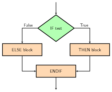
my_age, class_size to store a numbermy_name to store letters (a “string”)add_footer, for a function (action)TRUE/FALSE)IF condition THEN
do_task()
ELSE
do_something_else()
ENDIF

| A | B | A AND B | A OR B | NOT A |
|---|---|---|---|---|
| False | False | False | False | True |
| False | True | False | True | True |
| True | False | False | True | False |
| True | True | True | True | False |
if, else if and else{ and }{, RStudio does it for youn1 <- 11
n2 <- 7
if (n1 == n2) {
print(paste(n1, "and", n2, "are equal"))
} else if (n1 > n2) {
print(paste(n1, "is greater than", n2))
} else {
print(paste(n1, "is smaller than", n2))
}
[1] "11 is greater than 7"
We will see dplyr::case_when() for multiple if / else statements

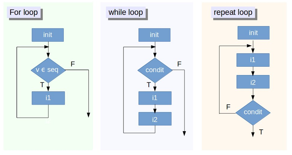
v <- c(3:7)
for (i in v) {
  print(i)
}
[1] 3
[1] 4
[1] 5
[1] 6
[1] 7
for (i in seq_along(v)) {
  print(paste("indice", i, "=", v[i]))
}
[1] "indice 1 = 3"
[1] "indice 2 = 4"
[1] "indice 3 = 5"
[1] "indice 4 = 6"
[1] "indice 5 = 7"
for_loop <- function(lgt) {
  res <- c()
  for (i in seq_len(lgt)) {
    res[i] <- i
  }
  length(res)
}for_loop_alloc <- function(lgt) {
res <- vector("integer", length = lgt)
for (i in seq_len(lgt)) {
res[i] <- i
}
length(res)
}Rcpplibrary(Rcpp)
cppFunction(
"NumericVector for_rcpp(int x) {
NumericVector res(x);
for (int i=0; i < x; i++) {
res[i] = i;
}
return res;
}")
@EmEmEff @quominus the slowness of for() loops is legendary: a mixture of history and fiction.
— Thomas Lumley (@tslumley) 12 June 2015

while and repeatExist in R but not covered in this course
In #rstats, it's surprisingly important to realise that names have objects; objects don't have names pic.twitter.com/bEMO1YVZX0
— Hadley Wickham (@hadleywickham) 16 May 2016
a <- matrix(0, ncol = 1000, nrow = 1000)
b <- a
a is ~ 8 Mb in RAMpryr::object_size(a) > 8 MB
b does not consume 16 Mb in RAMpryr::mem_change(b <- a) > 920 B
a or b are further altered, a copy is madepryr::mem_change(b[1, 1] <- 1) > 8 MB
source: David Smith on his blog
Everything that exists is an object. Everything that happens is a function call. John Chambers
The most important thing to understand about R is that functions are objects in their own right. You can work with them exactly the same way you work with any other type of object. Hadley Wickham, Advanced R
type names without ()
`+`
function (e1, e2) .Primitive("+")
is.infinite
function (x) .Primitive("is.infinite")1 + 2 * 3
[1] 7
`+`(1, `*`(2, 3))
[1] 7
sum(), sd()#library(purrr) map_dbl(women, sum)
height weight
   975   2051
<- and the keyword function to store a function in an object (name of function)f <- function() {}
f
function() {}f will not execute the code inside the function() i.e. f() in our examplef()
NULL
f() returns NULLbody(), the inside codeformals(), the list of argumentsenvironment(), location of the function’s variables.f <- function(x) x^2 f
function(x) x^2
formals(f) # assign is '='
$x
body(f)
x^2
environment(f)
<environment: R_GlobalEnv>
source: Hadley Wickham, Advanced R
f <- function() {
  print("Hello from biostat2!")
}f()f()
[1] "Hello from biostat2!"
f <- function() {
  1 + 1
  print("Hello from biostat2!")
  3 + 2
}
f()
[1] "Hello from biostat2!"
[1] 5
result <- f()
[1] "Hello from biostat2!"
# display the content
result
[1] 5
returnfunctions return the output of the last command
You can explicitly use the return() command to exit the function earlier and return a specified value
return() without argumentf <- function() {
1 + 1
3 + 2
}
f()[1] 5
f <- function() {
  1 + 1
  return()
  3 + 2
}
f()
NULL
return() with valuemakes function little useless
f <- function() {
  1 + 1
  return(6)
  3 + 2
}
f()
[1] 6
return() with variablemakes more sense
f <- function() {
  res <- 1 + 1
  return(res)
  3 + 2
}
f()
[1] 2
rm(z) # Removing any z object from global env
Warning in rm(z): object 'z' not found
f <- function(z) { # Note the 'z'
  z + 1
}

f()
Error in f(): argument "z" is missing, with no default
f(2)
[1] 3
rm(z)
Warning in rm(z): object 'z' not found
f <- function(z = 0) {
  z + 1
}

f()
[1] 1
f(2)
[1] 3
c’s?c <- 10 c(c = c)
c <- 10 assign scalar 10 to name c in global envc() concatenate function(c = c), 1st is named vector, 2nd is scalar (10)c <- 10 c(c = c)
 c
10
10c(c = c, use.names = FALSE)
[1] 10
ls() list loaded objectsls()
 [1] "a"       "average" "b"       "c"       "f"       "i"       "n1"
 [8] "n2"      "result"  "v"
ls() evaluated inside f()f <- function(x = ls()) {
a <- 1
x
}
f()
[1] "a" "x"
ls() evaluated in global environmentf(ls())
 [1] "a"       "average" "b"       "c"       "f"       "i"       "n1"
 [8] "n2"      "result"  "v"
source: Hadley Wickam Advanced R
Advanced topic, this is for your own knowledge!
Going back to our if, if else, else example and wrapping it in a function:
my_compare <- function(n1, n2) {
  if (n1 == n2) {
    message(paste(n1, "and", n2, "are equal"))
  } else if (n1 > n2) {
    message(paste(n1, "is greater than", n2))
  } else {
    message(paste(n1, "is smaller than", n2))
  }
}
my_compare(10, 10)
10 and 10 are equal
message("unnamed the arguments: R use order")unnamed the arguments: R use order
my_compare(2, 10)
2 is smaller than 10
my_compare(11, 10)
11 is greater than 10
message("named the arguments: safer")named the arguments: safer
my_compare(n1 = 11, n2 = 10)
11 is greater than 10
message("named arg allows you to switch them")named arg allows you to switch them
my_compare(n2 = 10, n1 = 11)
11 is greater than 10
1/0)my_function <- function(v) {
result <- v / 2;
print(result)
}
my_function(10)
[1] 5
my_function(TRUE)
[1] 0.5
my_function("a")
Error in v/2: non-numeric argument to binary operator
is.numeric(), is.character()stop(), warning()my_function <- function(v) {
if (!is.numeric(v)) {
stop("argument v should be a number!",
call. = FALSE)
}
result <- v / 2;
result
}
my_function(10)
[1] 5
my_function(TRUE)
Error: argument v should be a number!
my_function("a")
Error: argument v should be a number!
is_evenis_even <- function(n) {
if (!is.numeric(n)) {
stop("argument n should be a number!",
call. = FALSE)
}
if (length(n) == 0) {
stop("vector should contain at least 1 number",
call. = FALSE)
}
if (sum(is.na(n)) > 0) {
stop("vector should not contain missing data",
call. = FALSE)
}
n %% 2 == 0
}
is_even(integer(1))
[1] TRUE
is_even(NA_real_)
Error: vector should not contain missing data
