Rmarkdown and data import

September 2019

Rmarkdown

Learning objectives

You will learn to:

use the markdown syntax
create Rmarkdown documents
define the output format you expect to render
use the interactive RStudio interface to
- create your documents
- insert R code
- build your final document

RMarkdown

Why using `rmarkdown`?

write detailed reports
ensure reproducibility
keep track of your analyses
comment/describe each step of your analysis
export a single (Rmd) document to various formats (Pdf, Html…)
text file that can be managed by a version control system (like git)

Rmarkdown

+ +

Markdown

Markdown is used to format the text

Markup language

Such as Xml, HTML
A coding system used to structure text
Uses markup tags (e.g. <h1></h1> in HTML)

HTML

<!DOCTYPE html>
<html>
<body>

<h1>This is a heading</h1>

<p>This is some text in a paragraph.</p>

</body>
</html>

Lightweight markup language

Easy to read and write as it uses simple tags (e.g. #)

MD

# This is a heading

This is some text in a paragraph

Markdown

common text formatting tags

Headers

Levels are defined using #, ##, ### …

Text style

bold (**This will be bold**)
italic (*This will be italic*)

Links and images

http://example.com is auto-linked
[description](http://example.com)
![](path/to/image.jpg)

Verbatim code

code ( inline coding stuff )
triple backticks are delimiting code blocks

```
This is *verbatim* code
# Even headers are not interpreted
```

Rmarkdown cheatsheet

Have a look at the online documents on the Rmarkdown website
Use the Cheatsheet in the Help > Cheatsheets menu.

Exercise

Markdown

10:00

Learn to use the markdown syntax

Before writing your own Rmarkdown document, use the excellent ressource on commonmark.org to learn the basics of markdown formatting.

An alternative online ressource can be found on www.markdowntutorial.com

Including R code

Rmarkdown document

from the Rmarkdown cheatsheet

Rmarkdown

extends markdown
place R code in chunks
chunks will be evaluated
can also handle bash; python; css; …

Knitr

extracts R chunks
interprets them
formats results as markdown
reintegrates them into the main document (md)

Pandoc

pandoc converts markdown to the desired document (Pdf, Html, …)

Organising files

Use projects

The only two things that make @JennyBryan 😤😠🤯. Instead use projects + here::here() #rstats pic.twitter.com/GwxnHePL4n
— Hadley Wickham (@hadleywickham) December 11, 2017

Rstudio projects

Jennifer Bryan’s advice

Use here package to build paths

gets the root path of your project:
- detects Rstudio projects (.Rproj)
- git repository (.git)
- .here file

source: Jennifer Bryan’s article and test repo

RStudio projects

create

a new project
- in a new folder
- no git
create a sub-folder data
test here::here()
test here::dr_here()

Rmarkdown document

Create, step 1

Rmarkdown document

Create, step 2

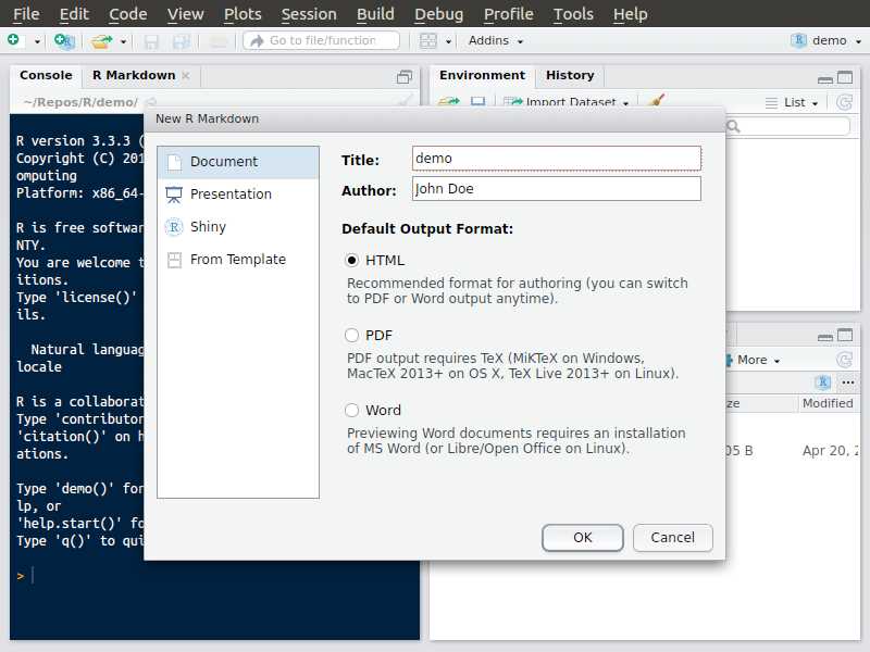
Rmarkdown document

Create, step 3

Generate your first HTML file

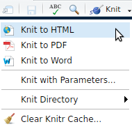
Use the knit button in RStudio

Rmarkdown document

Structure

YAML header

to define document wide options
title, name, …

markdown

markdown syntax to write your descriptions, remarks
litterate programming

chunks

code to be interpreted by R

R code chunks

Insert a chunk

R code chunks

delimited by triple backticks tags (```)
options in curly brackets
- engine evaluating the code
  R but also python, bash, …
- ```{r} is the minimum to define a starting R chunk
- name of chunk
- show or hide the source code
- evaluate it or not
- figure size …

R code chunks

navigate between different chunks

Inline R code

Integrate small pieces of R code

Use backticks ( ) followed by the keyword r:\ ``r ` ``

Example

Type in 1 + 1 = `r 1+1` to render 1 + 1 = 2.

Rmarkdown document

Generate the output document

use the integrated Knit button.
call rmarkdown::render()

Popular output formats

HTML

fast rendering
by default embeds binaries (pictures etc.)

PDF

single file
preserves original aspect
requires \(\LaTeX\)
have a look at the new TinyTeX package

Word document

widely used
easily editable
collaborate with people not using Rmarkdown
prepare scientific manuscripts suitable for submission

Bibliography

Supported formats

Use it with your EndNote or Zotero database:
BibLaTeX, BibTeX, EndNote, EndNote XML, MEDLINE, ISI, MODS, RIS, Copac, JSON citeproc

Styles

uses citation style language (csl) files
have a look at:
- https://www.zotero.org/styles
- https://github.com/citation-style-language/styles

Bibliography

How to

setup in the yaml header
insert citations using the pandoc syntax:
[@citation-key]

Example

---
title: "Sample Document"
output: html_document
bibliography: bibliography.bib
csl: nature.csl
---

Insert your reference [@my-reference] like I did.

Zotero

install the Better Bib(La)TeX plugin
adjust the preferences (for better integration)
export your database as bibtex
drag and drop pandoc keys to your Rmarkdown document

Import data using `readr`

Learning objectives

You will learn to:

use readr to import your data into R
use the interactive RStudio interface to visualise your data
appreciate tibbles

Importing data

Represents probably the first step of your work
R can handle multiple data types
- flat files (.csv, .tsv, …)
- excel files (.xls, .xlsx)
- foreign statistical formats (.sas from SAS, .sav from SPSS, .dta from Stata)
- databases (SQL, SQLite …)

Tidyverse implementation

R base already provides functions for text files (i.e. read.csv(), read.delim())
tidyverse redefines these functions:
- speed
- characters are not coerced to factors by default
- generates tibbles

Tibbles

have a refined print method that shows only the first 10 rows.
show all the columns that fit on screen and list the name of remaining ones.
each column reports its type.
makes it much easier to work with large data.

Hint

Use as_tibble() to convert a data.frame to a tibble

Tibbles

`tibble` vs `data.frame`

`data.frame`

iris

    Sepal.Length Sepal.Width Petal.Length Petal.Width    Species
1            5.1         3.5          1.4         0.2     setosa
2            4.9         3.0          1.4         0.2     setosa
3            4.7         3.2          1.3         0.2     setosa
4            4.6         3.1          1.5         0.2     setosa
5            5.0         3.6          1.4         0.2     setosa
6            5.4         3.9          1.7         0.4     setosa
7            4.6         3.4          1.4         0.3     setosa
8            5.0         3.4          1.5         0.2     setosa
9            4.4         2.9          1.4         0.2     setosa
10           4.9         3.1          1.5         0.1     setosa
11           5.4         3.7          1.5         0.2     setosa
12           4.8         3.4          1.6         0.2     setosa
13           4.8         3.0          1.4         0.1     setosa
14           4.3         3.0          1.1         0.1     setosa
15           5.8         4.0          1.2         0.2     setosa
16           5.7         4.4          1.5         0.4     setosa
17           5.4         3.9          1.3         0.4     setosa
18           5.1         3.5          1.4         0.3     setosa
19           5.7         3.8          1.7         0.3     setosa
20           5.1         3.8          1.5         0.3     setosa
21           5.4         3.4          1.7         0.2     setosa
22           5.1         3.7          1.5         0.4     setosa
23           4.6         3.6          1.0         0.2     setosa
24           5.1         3.3          1.7         0.5     setosa
25           4.8         3.4          1.9         0.2     setosa
26           5.0         3.0          1.6         0.2     setosa
27           5.0         3.4          1.6         0.4     setosa
28           5.2         3.5          1.5         0.2     setosa
29           5.2         3.4          1.4         0.2     setosa
30           4.7         3.2          1.6         0.2     setosa
31           4.8         3.1          1.6         0.2     setosa
32           5.4         3.4          1.5         0.4     setosa
33           5.2         4.1          1.5         0.1     setosa
34           5.5         4.2          1.4         0.2     setosa
35           4.9         3.1          1.5         0.2     setosa
36           5.0         3.2          1.2         0.2     setosa
37           5.5         3.5          1.3         0.2     setosa
38           4.9         3.6          1.4         0.1     setosa
39           4.4         3.0          1.3         0.2     setosa
40           5.1         3.4          1.5         0.2     setosa
41           5.0         3.5          1.3         0.3     setosa
42           4.5         2.3          1.3         0.3     setosa
43           4.4         3.2          1.3         0.2     setosa
44           5.0         3.5          1.6         0.6     setosa
45           5.1         3.8          1.9         0.4     setosa
46           4.8         3.0          1.4         0.3     setosa
47           5.1         3.8          1.6         0.2     setosa
48           4.6         3.2          1.4         0.2     setosa
49           5.3         3.7          1.5         0.2     setosa
50           5.0         3.3          1.4         0.2     setosa
51           7.0         3.2          4.7         1.4 versicolor
52           6.4         3.2          4.5         1.5 versicolor
53           6.9         3.1          4.9         1.5 versicolor
54           5.5         2.3          4.0         1.3 versicolor
55           6.5         2.8          4.6         1.5 versicolor
56           5.7         2.8          4.5         1.3 versicolor
57           6.3         3.3          4.7         1.6 versicolor
58           4.9         2.4          3.3         1.0 versicolor
59           6.6         2.9          4.6         1.3 versicolor
60           5.2         2.7          3.9         1.4 versicolor
61           5.0         2.0          3.5         1.0 versicolor
62           5.9         3.0          4.2         1.5 versicolor
63           6.0         2.2          4.0         1.0 versicolor
64           6.1         2.9          4.7         1.4 versicolor
65           5.6         2.9          3.6         1.3 versicolor
66           6.7         3.1          4.4         1.4 versicolor
67           5.6         3.0          4.5         1.5 versicolor
68           5.8         2.7          4.1         1.0 versicolor
69           6.2         2.2          4.5         1.5 versicolor
70           5.6         2.5          3.9         1.1 versicolor
71           5.9         3.2          4.8         1.8 versicolor
72           6.1         2.8          4.0         1.3 versicolor
73           6.3         2.5          4.9         1.5 versicolor
74           6.1         2.8          4.7         1.2 versicolor
75           6.4         2.9          4.3         1.3 versicolor
76           6.6         3.0          4.4         1.4 versicolor
77           6.8         2.8          4.8         1.4 versicolor
78           6.7         3.0          5.0         1.7 versicolor
79           6.0         2.9          4.5         1.5 versicolor
80           5.7         2.6          3.5         1.0 versicolor
81           5.5         2.4          3.8         1.1 versicolor
82           5.5         2.4          3.7         1.0 versicolor
83           5.8         2.7          3.9         1.2 versicolor
84           6.0         2.7          5.1         1.6 versicolor
85           5.4         3.0          4.5         1.5 versicolor
86           6.0         3.4          4.5         1.6 versicolor
87           6.7         3.1          4.7         1.5 versicolor
88           6.3         2.3          4.4         1.3 versicolor
89           5.6         3.0          4.1         1.3 versicolor
90           5.5         2.5          4.0         1.3 versicolor
91           5.5         2.6          4.4         1.2 versicolor
92           6.1         3.0          4.6         1.4 versicolor
93           5.8         2.6          4.0         1.2 versicolor
94           5.0         2.3          3.3         1.0 versicolor
95           5.6         2.7          4.2         1.3 versicolor
96           5.7         3.0          4.2         1.2 versicolor
97           5.7         2.9          4.2         1.3 versicolor
98           6.2         2.9          4.3         1.3 versicolor
99           5.1         2.5          3.0         1.1 versicolor
100          5.7         2.8          4.1         1.3 versicolor
101          6.3         3.3          6.0         2.5  virginica
102          5.8         2.7          5.1         1.9  virginica
103          7.1         3.0          5.9         2.1  virginica
104          6.3         2.9          5.6         1.8  virginica
105          6.5         3.0          5.8         2.2  virginica
106          7.6         3.0          6.6         2.1  virginica
107          4.9         2.5          4.5         1.7  virginica
108          7.3         2.9          6.3         1.8  virginica
109          6.7         2.5          5.8         1.8  virginica
110          7.2         3.6          6.1         2.5  virginica
111          6.5         3.2          5.1         2.0  virginica
112          6.4         2.7          5.3         1.9  virginica
113          6.8         3.0          5.5         2.1  virginica
114          5.7         2.5          5.0         2.0  virginica
115          5.8         2.8          5.1         2.4  virginica
116          6.4         3.2          5.3         2.3  virginica
117          6.5         3.0          5.5         1.8  virginica
118          7.7         3.8          6.7         2.2  virginica
119          7.7         2.6          6.9         2.3  virginica
120          6.0         2.2          5.0         1.5  virginica
121          6.9         3.2          5.7         2.3  virginica
122          5.6         2.8          4.9         2.0  virginica
123          7.7         2.8          6.7         2.0  virginica
124          6.3         2.7          4.9         1.8  virginica
125          6.7         3.3          5.7         2.1  virginica
126          7.2         3.2          6.0         1.8  virginica
127          6.2         2.8          4.8         1.8  virginica
128          6.1         3.0          4.9         1.8  virginica
129          6.4         2.8          5.6         2.1  virginica
130          7.2         3.0          5.8         1.6  virginica
131          7.4         2.8          6.1         1.9  virginica
132          7.9         3.8          6.4         2.0  virginica
133          6.4         2.8          5.6         2.2  virginica
134          6.3         2.8          5.1         1.5  virginica
135          6.1         2.6          5.6         1.4  virginica
136          7.7         3.0          6.1         2.3  virginica
137          6.3         3.4          5.6         2.4  virginica
138          6.4         3.1          5.5         1.8  virginica
139          6.0         3.0          4.8         1.8  virginica
140          6.9         3.1          5.4         2.1  virginica
141          6.7         3.1          5.6         2.4  virginica
142          6.9         3.1          5.1         2.3  virginica
143          5.8         2.7          5.1         1.9  virginica
144          6.8         3.2          5.9         2.3  virginica
145          6.7         3.3          5.7         2.5  virginica
146          6.7         3.0          5.2         2.3  virginica
147          6.3         2.5          5.0         1.9  virginica
148          6.5         3.0          5.2         2.0  virginica
149          6.2         3.4          5.4         2.3  virginica
150          5.9         3.0          5.1         1.8  virginica

Tibbles

`tibble` vs `data.frame`

`tibble`

# library(tibble)
as_tibble(iris)

# A tibble: 150 x 5
   Sepal.Length Sepal.Width Petal.Length Petal.Width Species
          <dbl>       <dbl>        <dbl>       <dbl> <fct>  
 1          5.1         3.5          1.4         0.2 setosa 
 2          4.9         3            1.4         0.2 setosa 
 3          4.7         3.2          1.3         0.2 setosa 
 4          4.6         3.1          1.5         0.2 setosa 
 5          5           3.6          1.4         0.2 setosa 
 6          5.4         3.9          1.7         0.4 setosa 
 7          4.6         3.4          1.4         0.3 setosa 
 8          5           3.4          1.5         0.2 setosa 
 9          4.4         2.9          1.4         0.2 setosa 
10          4.9         3.1          1.5         0.1 setosa 
# … with 140 more rows

`tibble` adjusts to width

# A tibble: 150 x 5
   Sepal.Length Sepal.Width
          <dbl>       <dbl>
 1          5.1         3.5
 2          4.9         3  
 3          4.7         3.2
 4          4.6         3.1
 5          5           3.6
 6          5.4         3.9
 7          4.6         3.4
 8          5           3.4
 9          4.4         2.9
10          4.9         3.1
# … with 140 more rows, and 3
#   more variables:
#   Petal.Length <dbl>,
#   Petal.Width <dbl>,
#   Species <fct>

tibble printing enhancements

column type is visible
shows only the first 10 rows
shows only the columns that fit on the screen

Create tibbles

`tibble()`

similar to base::data.frame() but
- does not coerce characters to factors
- does not change column names
- never uses rownames

data.frame(`bad name` = 1:4,
           x = rep(letters[1:2], 2)) %>%
  str()

'data.frame':   4 obs. of  2 variables:
 $ bad.name: int  1 2 3 4
 $ x       : Factor w/ 2 levels "a","b": 1 2 1 2

tibble(`bad name` = 1:4,
       x = rep(letters[1:2], 2)) %>%
  str()

Classes 'tbl_df', 'tbl' and 'data.frame':   4 obs. of  2 variables:
 $ bad name: int  1 2 3 4
 $ x       : chr  "a" "b" "a" "b"

The tidyverse packages to import your data

Tidyverse packages to import your data

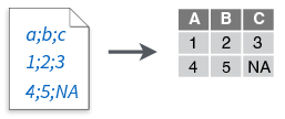
Seven file formats are supported by the readr package:

read_csv(): comma separated (CSV) files
read_tsv(): tab separated files
read_delim(): general delimited files
read_fwf(): fixed width files
read_table(): tabular files where colums are separated by white-space.
read_log(): web log files

`readxl`

To import excel files (.xls and .xlsx):

read_excel()
- read_xls()
- read_xlsx()

haven

read_sas() for SAS
read_sav() for SPSS
read_dta() for Stata

Importing flat files

Reading flat files

Flat file example: mtcars.csv

Create a new project (finding your files will be easier)
Download the mtcars.csv file to your project folder (using your favourite browser)
Open the file with a text viewer and have a look at its content

"mpg","cyl","disp","hp","drat","wt","qsec","vs","am","gear","carb"
21,6,160,110,3.9,2.62,16.46,0,1,4,4
21,6,160,110,3.9,2.875,17.02,0,1,4,4
22.8,4,108,93,3.85,2.32,18.61,1,1,4,1
21.4,6,258,110,3.08,3.215,19.44,1,0,3,1
18.7,8,360,175,3.15,3.44,17.02,0,0,3,2
...

Rstudio data import

interactive call to `readr`

Import button

Use the Import Dataset button in the upper right panel or click on the file in the lower right panel

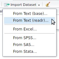
Will interactively select the appropriate function
Copy paste the generated command to your Rmarkdown document

Exercise

Import the `mtcars.csv` dataset

Use the interactive Import Dataset button to import the mtcars.csv file.

Rstudio data import

preview window

Reading flat files

comma separated values

`read_csv()`

to import comma separated values
is able to read local and remote files
is able to read compressed files (.zip, .gz, …)

Reading flat files

comma separated values

Using `read_csv()`

read_csv(here::here("data", "mtcars.csv"))

Parsed with column specification:
cols(
  mpg = col_double(),
  cyl = col_double(),
  disp = col_double(),
  hp = col_double(),
  drat = col_double(),
  wt = col_double(),
  qsec = col_double(),
  vs = col_double(),
  am = col_double(),
  gear = col_double(),
  carb = col_double()
)

# A tibble: 32 x 11
     mpg   cyl  disp    hp  drat    wt  qsec    vs    am  gear  carb
   <dbl> <dbl> <dbl> <dbl> <dbl> <dbl> <dbl> <dbl> <dbl> <dbl> <dbl>
 1  21       6  160    110  3.9   2.62  16.5     0     1     4     4
 2  21       6  160    110  3.9   2.88  17.0     0     1     4     4
 3  22.8     4  108     93  3.85  2.32  18.6     1     1     4     1
 4  21.4     6  258    110  3.08  3.22  19.4     1     0     3     1
 5  18.7     8  360    175  3.15  3.44  17.0     0     0     3     2
 6  18.1     6  225    105  2.76  3.46  20.2     1     0     3     1
 7  14.3     8  360    245  3.21  3.57  15.8     0     0     3     4
 8  24.4     4  147.    62  3.69  3.19  20       1     0     4     2
 9  22.8     4  141.    95  3.92  3.15  22.9     1     0     4     2
10  19.2     6  168.   123  3.92  3.44  18.3     1     0     4     4
# … with 22 more rows

Column types

are guessed from the 1000 first rows
- adjustable guess_max option
guessed types are displayed as a message
to hide this message:
- lazy method 1: set message = FALSE in your rmarkdown chunk option.
- lazy method 2: set col_types = cols()
- Hadley Wickham recommends to adjust the col_types to avoid any problem

Message

Parsed with column specification:
cols(
  mpg = col_double(),
  cyl = col_double(),
  disp = col_double(),
  hp = col_double(),
  drat = col_double(),
  wt = col_double(),
  qsec = col_double(),
  vs = col_double(),
  am = col_double(),
  gear = col_double(),
  carb = col_double()
)

Column types

The `col_types` argument

exa <- here::here("data", "example.csv")

read_csv(exa, col_types = cols())

# A tibble: 3 x 3
  animal  colour value
  <chr>   <chr>  <dbl>
1 dog     red        1
2 cat     blue       2
3 chicken green      6

Let’s start with a file containing only 3 columns: animal, colour and value
Column types are specified using the cols() function
Types can be one of double, integer, character, logical, factor, date, datetime or time

Column types

Explicit method

Using a function defining each type:

col_double()
col_integer()
col_character()
col_logical()
col_factor()
col_date()
col_datetime()
col_time()

Or telling to guess or skip a column:

col_guess()
col_skip()

Example

read_csv(exa,
         col_types = cols(
           animal = col_character(),
           colour = col_character(),
           value = col_integer()
         ))

# A tibble: 3 x 3
  animal  colour value
  <chr>   <chr>  <int>
1 dog     red        1
2 cat     blue       2
3 chicken green      6

Column types

Compact shortcuts

Using a single character to define each type:

c = character
i = integer
n = number
d = double
l = logical
D = date
T = date time
t = time

Or telling to guess or skip a column:

? = guess
_ or - = skip

Example

read_csv(exa,
         col_types = cols(
           animal = "c",
           colour = "c",
           value = "i"
         ))

# A tibble: 3 x 3
  animal  colour value
  <chr>   <chr>  <int>
1 dog     red        1
2 cat     blue       2
3 chicken green      6

Even more compact

read_csv(exa, col_types = "cci")

Use the single character code in the order of appearance of each column

Exercise

Override the detected column types

import the example.csv file but
- skip the colour column
- read in the value column as double

Exercise

Answer

read_csv(exa, col_types = cols(animal = col_character(),
                               colour = col_skip(),
                               value = col_double()))

# A tibble: 3 x 2
  animal  value
  <chr>   <dbl>
1 dog         1
2 cat         2
3 chicken     6

read_csv(exa, col_types = cols(animal = "c",
                               colour = "_",
                               value = "d"))

# A tibble: 3 x 2
  animal  value
  <chr>   <dbl>
1 dog         1
2 cat         2
3 chicken     6

read_csv(exa, col_types = "c_d")

# A tibble: 3 x 2
  animal  value
  <chr>   <dbl>
1 dog         1
2 cat         2
3 chicken     6

Column names

The `col_names` argument

can be either TRUE, FALSE or a character vector.
default value is TRUE
if TRUE, the first row will be used as column names
if FALSE, names are generated (X1, X2, X3, …)
if it is a character vector, it will define the column names

Example

read_csv(exa,
         col_names = TRUE)

# A tibble: 3 x 3
  animal  colour value
  <chr>   <chr>  <dbl>
1 dog     red        1
2 cat     blue       2
3 chicken green      6

read_csv(exa,
         col_names = FALSE)

# A tibble: 4 x 3
  X1      X2     X3   
  <chr>   <chr>  <chr>
1 animal  colour value
2 dog     red    1    
3 cat     blue   2    
4 chicken green  6

read_csv(exa,
         col_names = c("name", "colname", "number"))

# A tibble: 4 x 3
  name    colname number
  <chr>   <chr>   <chr> 
1 animal  colour  value 
2 dog     red     1     
3 cat     blue    2     
4 chicken green   6

Column names

Hint

col_names is handy if they are no column names in the file
If you would like to rename columns, use dplyr::rename() (see upcoming dplyr lecture).

read_csv(exa, col_names = c("name", "colname", "number"))

# A tibble: 4 x 3
  name    colname number
  <chr>   <chr>   <chr> 
1 animal  colour  value 
2 dog     red     1     
3 cat     blue    2     
4 chicken green   6

read_csv(exa, col_names = TRUE) %>%
  rename(name = animal,
         colname = colour,
         number = value)

# A tibble: 3 x 3
  name    colname number
  <chr>   <chr>    <dbl>
1 dog     red          1
2 cat     blue         2
3 chicken green        6

Skipping lines

`skip` argument

To skip the first n rows

`n_max` argument

To stop reading after n rows

Hint

You might want to adjust col_names to get what you want

readr_example("mtcars.csv") %>%
  read_csv(skip = 3,
           n_max = 3,
           col_names = FALSE)

# A tibble: 3 x 11
     X1    X2    X3    X4    X5    X6    X7    X8    X9   X10   X11
  <dbl> <dbl> <dbl> <dbl> <dbl> <dbl> <dbl> <dbl> <dbl> <dbl> <dbl>
1  22.8     4   108    93  3.85  2.32  18.6     1     1     4     1
2  21.4     6   258   110  3.08  3.22  19.4     1     0     3     1
3  18.7     8   360   175  3.15  3.44  17.0     0     0     3     2

readr_example("mtcars.csv") %>%
  read_csv(skip = 3, n_max = 3,
           col_names = c("mpg", "cyl", "disp", "hp", "drat", "wt", "qsec", "vs", "am", "gear", "carb"))

# A tibble: 3 x 11
    mpg   cyl  disp    hp  drat    wt  qsec    vs    am  gear  carb
  <dbl> <dbl> <dbl> <dbl> <dbl> <dbl> <dbl> <dbl> <dbl> <dbl> <dbl>
1  22.8     4   108    93  3.85  2.32  18.6     1     1     4     1
2  21.4     6   258   110  3.08  3.22  19.4     1     0     3     1
3  18.7     8   360   175  3.15  3.44  17.0     0     0     3     2

`readr` functions

`read_csv()`

Comma delimited files

`read_csv2()`

Semi-colon delimited files

`read_tsv()`

tab delimited files

`read_delim()`

any delimiter:

read_delim(file, delim = "|", ...)

`read_fwf()`

fixed width files

If speed is still an issue

`fread` from `data.table`

stable
install.packages("data.table")
overhauled
2X faster than readr

promising `vroom`

on CRAN
install.packages("vroom")
by Jim Hester (readr)
same syntax!
multi-threaded
ALTREP framework
18X faster than readr in some conditions

Wrap up

You learned to:

appreciate the tibble printing features
- column types are displayed
use readr to import your flat file data into R
- using the command line
- using the interactive RStudio interface
adjust the imported data types

Before we stop

Acknowledgments

Hadley Wickham

Rmarkdown

Learning objectives

You will learn to:

RMarkdown

Why using rmarkdown?

Rmarkdown

Markdown

Markup language

HTML

Lightweight markup language

MD

Markdown

common text formatting tags

Headers

Text style

Links and images

Verbatim code

Rmarkdown cheatsheet

Exercise

Markdown

Learn to use the markdown syntax

Including R code

Rmarkdown document

Rmarkdown

Knitr

Pandoc

Organising files

Use projects

Rstudio projects

Jennifer Bryan’s advice

RStudio projects

create

Rmarkdown document

Create, step 1

Rmarkdown document

Create, step 2

Rmarkdown document

Create, step 3

Generate your first HTML file

Rmarkdown document

Structure

YAML header

markdown

chunks

R code chunks

Insert a chunk

R code chunks

R code chunks

navigate between different chunks

Inline R code

Integrate small pieces of R code

Example

Rmarkdown document

Generate the output document

Popular output formats

HTML

PDF

Word document

Bibliography

Supported formats

Styles

Bibliography

How to

Example

Zotero

Import data using readr

Learning objectives

You will learn to:

Importing data

Tidyverse implementation

Tibbles

Tibbles

Hint

Tibbles

tibble vs data.frame

data.frame

Tibbles

tibble vs data.frame

tibble

tibble adjusts to width

Why using `rmarkdown`?

Import data using `readr`

`tibble` vs `data.frame`

`data.frame`

`tibble` vs `data.frame`

`tibble`

`tibble` adjusts to width

`tibble()`

`readxl`

interactive call to `readr`

Import the `mtcars.csv` dataset

`read_csv()`

Using `read_csv()`

The `col_types` argument

The `col_names` argument

`skip` argument

`n_max` argument

`readr` functions

`read_csv()`

`read_csv2()`

`read_tsv()`

`read_delim()`

`read_fwf()`

`fread` from `data.table`

promising `vroom`